---
title: "Koopman unrolling — learning eigenfunctions from data"
author: "Etienne Meunier"
date: today
format:
html:
number-sections: true
code-fold: show
code-tools: true
---
In the previous tutorials we found Koopman eigenfunctions by hand. Here everything is learned from data: encoder, dynamic and decoder are trained jointly with a single objective:
$$
\min_{A, \mathcal E, \mathcal D} \; \mathbb E_{(t_0, t)} \, \big|\big| x_{t} - \mathcal D\big(e^{A (t - t_0)}\,\mathcal E(x_{t_0})\big)\big|\big|_2^2
$$
Each block matches an object from the [introduction](koopman-introduction.qmd):
- encoder $\mathcal E$ — the eigenfunctions
- $A$ — the eigenvalues
- decoder $\mathcal D$ — the modes for reconstruction
::: {.callout-note collapse="true"}
## Why "unrolling"?
Discrete-time methods learn an operator $K$ and iterate it: $z_{t+n} = K^n z_t$, backpropagating through the unrolled product. In continuous time $e^{A(t - t_0)}$ is a single closed-form matrix — any gap works: irregular, off-grid, even negative.
:::
Two design choices follow: the dynamic and the decoder.
# The dynamic
Two visions:
- **pure Koopman** — each eigenfunction is a complex number, driven by an eigenvalue $\lambda \in \mathbb C$
- **dense** — a multi-dimensional latent driven by a dense matrix $A$ (common in deep learning papers). A dense $A$ is fine: it just couples the latent dimensions.
Our mental image for this tutorial:
{fig-align="center"}
$j$ independent modes, each of dimension $l$. Stacked, the full latent dynamic is block-diagonal: $j$ blocks of size $l \times l$. The encoder maps $x \in \mathbb R^p$ to $z \in \mathbb R^{j \times l}$.
```{python}
#| label: imports
#| code-fold: true
#| code-summary: "Show imports"
import torch
import torch.nn as nn
import torch.nn.functional as F
from torchdiffeq import odeint
from dataclasses import dataclass
from einops import einsum as es, rearrange, repeat
import matplotlib.pyplot as plt

torch.manual_seed(0)
```
```{python}
#| label: dynamics
#| code-fold: true
#| code-summary: "Show dynamics code"
class Dynamics(nn.Module):
    """
        Represent a set of j independent dynamics,
        each acting (in parallel, independently)
        on a state of dimension l.
    """
    def __init__(self, j, l):
        super().__init__()
        self.j, self.l = j, l

    def propagate(self, t0, z0, t):
        """
            Propagate the points starting from (t0, z0)
            using the dynamic and return their value at times t

            Params :
                t0 (b)     : reference time
                z0 (b j l) : reference state
                t (b k)    : times to sample

            Return :
                z (b k j l) : propagated states
        """
        raise NotImplementedError


class Dense(Dynamics):
    """
        Each dynamic is represented as a dense l,l matrix
    """
    def __init__(self, j, l):
        super().__init__(j, l)
        self.A = nn.Parameter(torch.randn(self.j, self.l, self.l))

    def propagate(self, t0, z0, t):
        dts = t - t0[:, None]  # (b, k)
        Adts = es(dts, self.A, 'b k, j v l -> b k j v l')
        eA = torch.matrix_exp(Adts)  # (b k j v l)
        z = es(eA, z0, 'b k j v l, b j l -> b k j v')
        return z


class ScalingRotation2D(Dynamics):
    """
        Each dynamic is a 2x2 block representing a scaling and a rotation.
        Parameters are just the factors of this scaling and rotation;
        this corresponds to the "pure" Koopman approach
        with complex eigenfunctions.
    """
    def __init__(self, j, l):
        assert l == 2, 'l needs to be 2 for scaling rotation dynamics'
        super().__init__(j, l)
        self.gamma = nn.Parameter(torch.randn(self.j))
        self.omega = nn.Parameter(torch.randn(self.j))
        # constants: registered as buffers so they follow .to(device) but aren't trained
        self.register_buffer('J', torch.tensor([[0., -1.], [1., 0.]]))
        self.register_buffer('I', torch.eye(2))

    def matrix_exp_Adt(self, dt):
        """
            Compute e^{A dt} per 2x2 block

            Params :
                dt (b k) : gaps we want to compute
            Returns :
                blocks_exp (b k j 2 2) : matrix exponential per block
        """
        arg_g = es(dt, self.gamma, 'b k, j -> b k j')  # (b k j)
        arg_o = es(dt, self.omega, 'b k, j -> b k j')  # (b k j)
        eg, co, so = torch.exp(arg_g), torch.cos(arg_o), torch.sin(arg_o)  # (b k j)
        rot = es(co, self.I, 'b k j, d c -> b k j d c') \
            + es(so, self.J, 'b k j, d c -> b k j d c')  # (b k j 2 2)
        blocks_exp = es(eg, rot, 'b k j, b k j d c -> b k j d c')  # (b k j 2 2)
        return blocks_exp

    def propagate(self, t0, z0, t):
        dts = t - t0[:, None]  # (b, k)
        eA = self.matrix_exp_Adt(dts)  # (b k j 2 2)
        z = es(eA, z0, 'b k j d l, b j l -> b k j d')
        return z
```
The 2D scaling-rotation block has a closed-form exponential — super cheap:
$$
\dot z = (\gamma I + \omega J)z \;\text{ with }\; J = \begin{bmatrix} 0 & -1 \\ 1 & 0\end{bmatrix} \;\to\; z(t) = e^{(\gamma I + \omega J)t}z_0 = e^{\gamma t} \begin{bmatrix} \cos \omega t & -\sin \omega t \\ \sin \omega t & \cos \omega t \end{bmatrix} z_0
$$
This is exactly the polar form of the [complex example](koopman-nonlinear-complex-example.qmd): $(\gamma, \omega)$ are the real and imaginary parts of the eigenvalue, and each 2D block holds a complex eigenfunction together with its conjugate.
::: {.callout-note collapse="true"}
## Dense vs. scaling-rotation: same expressivity
A real dense $A$ is diagonalizable over $\mathbb C$, eigenvalues in conjugate pairs. The encoder and decoder can absorb the change of basis, so dense blocks and scaling-rotation blocks are equivalent in expressivity. The difference is the optimization landscape and the cost of the exponential.
:::
# The decoder
Two options:
- **linear** — each observation is a linear combination of eigenfunctions, the "pure" Koopman reconstruction:
$$
x \approx \sum_j \kern1pt v_j^\top \, z_j
$$
- **MLP** — common in deep learning; a linear decoder may need a very large set of eigenfunctions for realistic dynamics.
```{python}
#| label: coders
#| code-fold: true
#| code-summary: "Show encoder / decoder code"
def mlp(sizes, activation=nn.GELU):
    """Plain MLP: Linear/activation stack, no activation after the last layer."""
    layers = []
    for i in range(len(sizes) - 1):
        layers.append(nn.Linear(sizes[i], sizes[i + 1]))
        if i < len(sizes) - 2:
            layers.append(activation())
    return nn.Sequential(*layers)


class MLPEncoder(nn.Module):
    """
        Map a physical state x in R^p to j independent modes, each of dim l.
        x (b, p) -> z (b, j, l)
    """
    def __init__(self, p, j, l, hidden=(128, 128)):
        super().__init__()
        self.j, self.l = j, l
        self.net = mlp([p, *hidden, j * l])

    def forward(self, x):
        z = self.net(x)  # (b, j*l)
        return rearrange(z, 'b (j l) -> b j l', j=self.j, l=self.l)


class LinearDecoder(nn.Module):
    """
        Linear combination of the modes: z (..., j, l) -> x (..., p).
        This is the "pure" Koopman reconstruction.
    """
    def __init__(self, p, j, l, bias=False):
        super().__init__()
        self.V = nn.Linear(j * l, p, bias=bias)

    def forward(self, z):
        return self.V(rearrange(z, '... j l -> ... (j l)'))


class MLPDecoder(nn.Module):
    """Non-linear decoder: z (..., j, l) -> x (..., p)."""
    def __init__(self, p, j, l, hidden=(128, 128)):
        super().__init__()
        self.net = mlp([j * l, *hidden, p])

    def forward(self, z):
        return self.net(rearrange(z, '... j l -> ... (j l)'))
```
# Example: learning an eigenfunction representation
The "classical" Koopman case: 2D scaling-rotation dynamic + linear reconstruction.
## Data and simulation
Same system as the [complex example](koopman-nonlinear-complex-example.qmd) — we know its spectrum analytically:
- $\psi(x) = x_1 + i(x_2 - c\,x_1^2)$, eigenvalue $(\gamma, \omega) = (1, 4)$
- exact linear reconstruction from the lattice: $\psi^2 \to (2, 8)$ and $\psi\bar\psi \to (2, 0)$
So after training we can check whether the optimizer rediscovers this spectrum.
```{python}
#| label: system
@dataclass
class ComplexPoint:
    a: float
    c: float
    w: float

    def f(self, t, x):
        """x (..., 2) -> dx/dt (..., 2)"""
        x1, x2 = x[..., 0], x[..., 1]
        xp1 = self.a * x1 - self.w * x2 + self.w * self.c * x1**2
        xp2 = (
            self.w * x1
            + self.a * x2
            + self.a * self.c * x1**2
            - 2 * self.c * self.w * x1 * x2
            + 2 * self.c**2 * self.w * x1**3
        )
        return torch.stack([xp1, xp2], dim=-1)

fp = ComplexPoint(1.0, 3.0, 4.0)
```
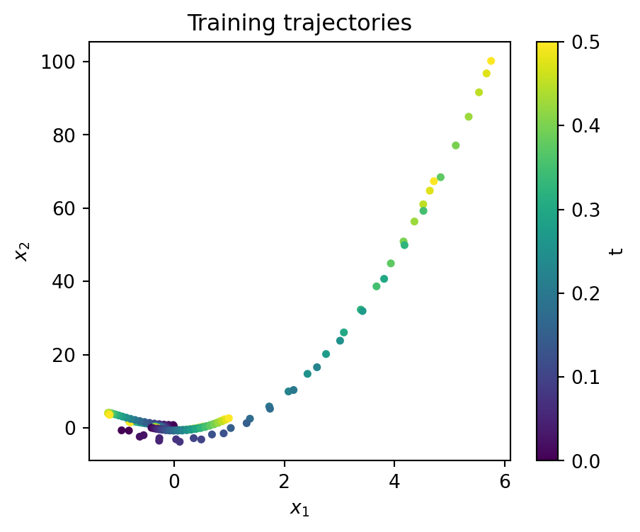
We integrate trajectories from random initial states, observed on a regular grid. Nothing in the model requires the grid to be regular.
```{python}
#| label: data
N_TRAIN, N_VAL = 300, 50
T_SPAN, N_T    = 0.5, 21

t_grid = torch.linspace(0, T_SPAN, N_T)               # (T)
x0s    = torch.rand(N_TRAIN + N_VAL, 2) * 2 - 1       # (N, 2) in [-1, 1]^2
trajs  = odeint(fp.f, x0s, t_grid).transpose(0, 1)    # (N, T, 2)
x_train, x_val = trajs[:N_TRAIN], trajs[N_TRAIN:]
```
```{python}
#| label: fig-data
#| fig-cap: "A few training trajectories in state space, colored by time."
#| code-fold: true
#| code-summary: "Show plotting code"
plt.figure(figsize=(5, 4))
for k in range(8):
    sc = plt.scatter(*x_train[k].T, c=t_grid, s=10)
plt.xlabel(r"$x_1$")
plt.ylabel(r"$x_2$")
plt.colorbar(sc, label="t")
plt.title("Training trajectories")
plt.show()
```
## Training
The three blocks assemble into $\tilde x_t = \mathcal D(e^{A(t - t_0)} \mathcal E(x_{t_0}))$:
```{python}
#| label: model
class KoopmanModel(nn.Module):
    """
        Encode a reference state, propagate it with the latent dynamic
        up to the requested times, decode back to physical space.
    """
    def __init__(self, encoder, dynamic, decoder):
        super().__init__()
        self.encoder, self.dynamic, self.decoder = encoder, dynamic, decoder

    def forward(self, t0, x0, t):
        """
            Params :
                t0 (b)    : reference times
                x0 (b p)  : reference states
                t (b k)   : times we want to predict
            Return :
                x (b k p) : predicted states
        """
        z0 = self.encoder(x0)                   # (b j l)
        z  = self.dynamic.propagate(t0, z0, t)  # (b k j l)
        return self.decoder(z)                  # (b k p)


P, J_MODES, L_DIM = 2, 8, 2

model = KoopmanModel(
    encoder = MLPEncoder(P, J_MODES, L_DIM),
    dynamic = ScalingRotation2D(J_MODES, L_DIM),
    decoder = LinearDecoder(P, J_MODES, L_DIM),
)
```
Training loop:
- each trajectory gets a **random** reference point $(t_0, x_{t_0})$
- we supervise the prediction at every observed time
- negative gaps included — backwards propagation comes for free with the matrix exponential
```{python}
#| label: training
def unroll_loss(model, x, t_grid):
    """Random reference point per trajectory, predict the whole trajectory."""
    b = x.shape[0]
    i0 = torch.randint(0, x.shape[1], (b,))
    t0, x0 = t_grid[i0], x[torch.arange(b), i0]  # (b), (b p)
    t = repeat(t_grid, 'k -> b k', b=b)          # (b k)
    return F.mse_loss(model(t0, x0, t), x)


opt = torch.optim.Adam(model.parameters(), lr=1e-3)
BATCH, STEPS = 100, 5000

logs = {'step': [], 'train': [], 'val': []}
for step in range(STEPS + 1):
    idx  = torch.randint(0, N_TRAIN, (BATCH,))
    loss = unroll_loss(model, x_train[idx], t_grid)
    opt.zero_grad(); loss.backward(); opt.step()

    if step % 100 == 0:
        with torch.no_grad():
            val = unroll_loss(model, x_val, t_grid)
        logs['step'].append(step)
        logs['train'].append(loss.item())
        logs['val'].append(val.item())

print(f"final train {logs['train'][-1]:.4f}  val {logs['val'][-1]:.4f}")
```
```{python}
#| label: fig-loss
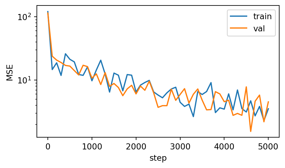
#| fig-cap: "Training and validation loss."
#| code-fold: true
#| code-summary: "Show plotting code"
plt.figure(figsize=(5, 3))
plt.plot(logs['step'], logs['train'], label='train')
plt.plot(logs['step'], logs['val'], label='val')
plt.yscale('log')
plt.xlabel('step')
plt.ylabel('MSE')
plt.legend()
plt.tight_layout()
plt.show()
```
## Inference
Propagate an initial condition with the trained blocks:
$$
\tilde x(t) = \mathcal D\big(e^{At}\,\mathcal E(x(0))\big)
$$
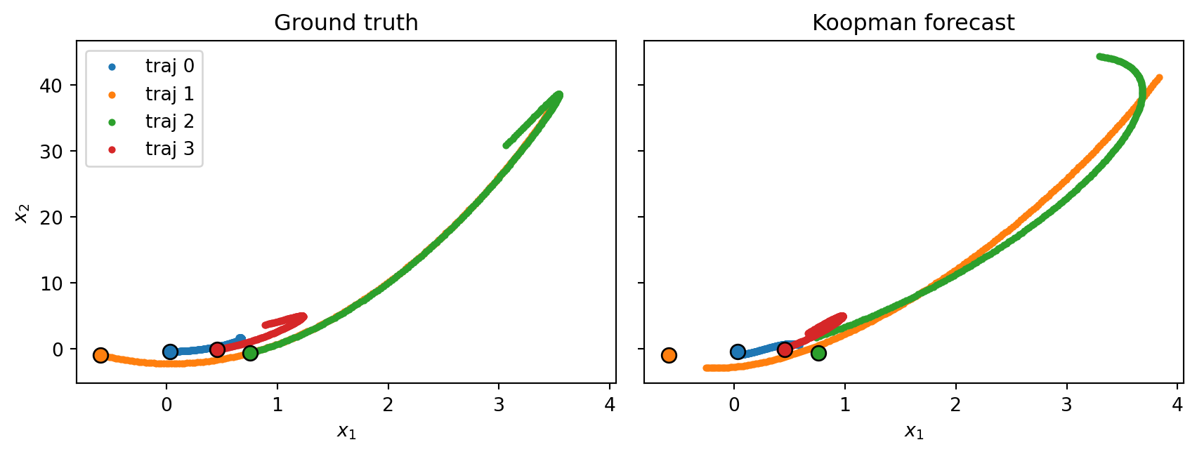
We compare against the true integration from unseen initial states, on a grid **10x finer** than training — the continuous formulation predicts at times it never saw.
```{python}
#| label: forecast
x0_test = torch.rand(4, 2) * 2 - 1
t_fine  = torch.linspace(0, T_SPAN, 200)

with torch.no_grad():
    gt   = odeint(fp.f, x0_test, t_fine).transpose(0, 1)              # (4, 200, 2)
    t_pred = repeat(t_fine, 'k -> b k', b=len(x0_test))
    pred   = model(torch.zeros(len(x0_test)), x0_test, t_pred)        # (4, 200, 2)
```
```{python}
#| label: fig-forecast
#| fig-cap: "True integration (left) vs. Koopman forecast (right) from unseen initial states (marked in black), on a time grid 10x finer than training."
#| code-fold: true
#| code-summary: "Show plotting code"
fig, axs = plt.subplots(1, 2, figsize=(9, 3.5), sharex=True, sharey=True)
axs[0].set_title("Ground truth")
axs[1].set_title("Koopman forecast")

for k in range(len(x0_test)):
    color = f"C{k}"
    axs[0].scatter(*gt[k].T, s=8, color=color, label=f"traj {k}")
    axs[1].scatter(*pred[k].T, s=8, color=color)
    for ax in axs:
        ax.scatter(*x0_test[k], color=color, edgecolors="k", s=60, zorder=3)

axs[0].legend()
for ax in axs:
    ax.set_xlabel(r"$x_1$")
axs[0].set_ylabel(r"$x_2$")
fig.tight_layout()
plt.show()
```
## Did we recover the spectrum?
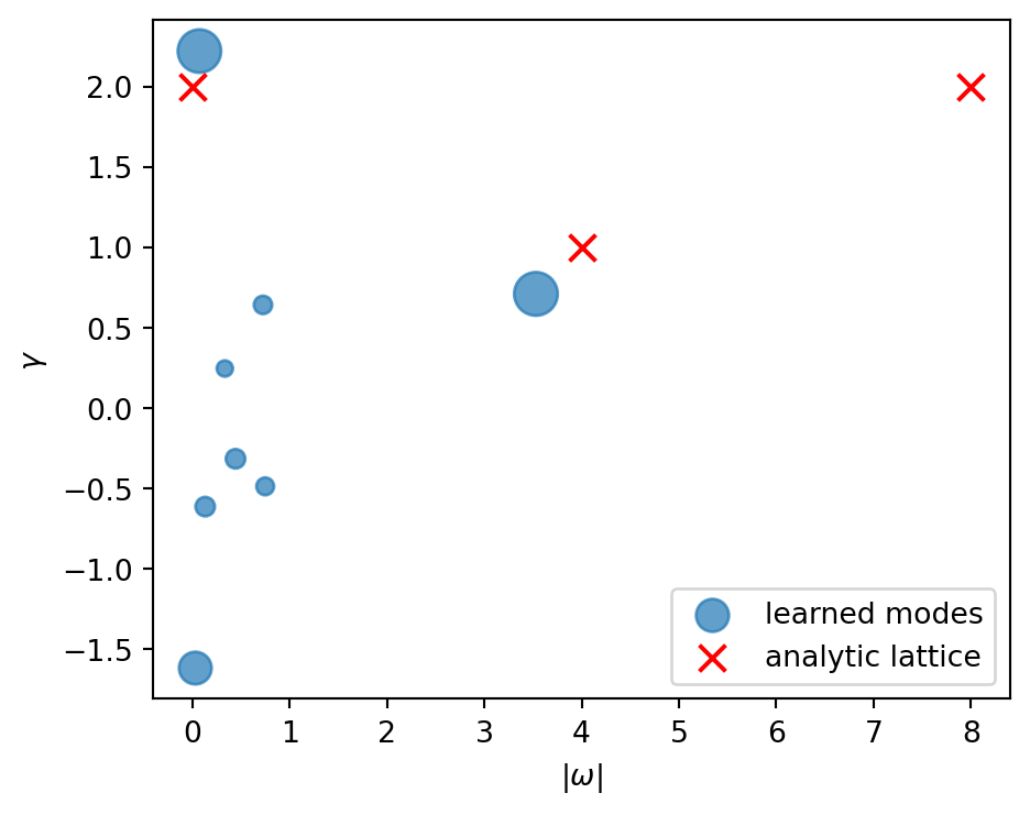
Each mode carries a readable eigenvalue $\lambda_j = \gamma_j + i\,\omega_j$, to compare against the analytic lattice $(1, 4), (2, 8), (2, 0)$. Two details:
- the sign of $\omega_j$ is a conjugacy — we look at $|\omega_j|$
- unused modes receive no training signal — we weight each mode by its contribution to the reconstruction (*usage*)
```{python}
#| label: spectrum
gamma = model.dynamic.gamma.detach()
omega = model.dynamic.omega.detach().abs()

# usage: RMS of each mode's contribution to the reconstruction over val states
with torch.no_grad():
    z  = model.encoder(rearrange(x_val, 'n t p -> (n t) p'))  # (nt, j, l)
    Vb = rearrange(model.decoder.V.weight, 'p (j l) -> j p l', j=J_MODES)
    contrib = es(Vb, z, 'j p l, n j l -> n j p')              # (nt, j, p)
    usage   = contrib.norm(dim=-1).pow(2).mean(0).sqrt()      # (j)

for jj in usage.argsort(descending=True):
    print(f"mode {jj}:  gamma {gamma[jj]: .2f}   |omega| {omega[jj]:.2f}   usage {usage[jj]:.2f}")
```
::: {.callout-note collapse="true"}
## How the usage is computed
The linear decoder splits the reconstruction into per-mode contributions:
$$
\tilde x = V z = \sum_j V_j\, z_j
\qquad\qquad
\text{usage}_j = \sqrt{\;\mathbb E_x\big[\,||V_j\, z_j(x)||_2^2\,\big]\;}
$$
- we must measure the *product* $V_j z_j$: weights or latents alone are meaningless, the model can rescale one and compensate in the other ($z_j \to \alpha z_j$, $V_j \to V_j / \alpha$)
- usage $\approx 0$ means no training signal on $(\gamma_j, \omega_j)$: the mode can sit anywhere on the spectrum plot
:::
```{python}
#| label: fig-spectrum
#| fig-cap: "Learned spectrum: each dot is a mode, sized by its contribution to the reconstruction. Red crosses mark the analytic eigenvalues of the lattice."
#| code-fold: true
#| code-summary: "Show plotting code"
plt.figure(figsize=(5, 4))
plt.scatter(omega, gamma, s=20 + 200 * usage / usage.max(), alpha=0.7, label='learned modes')
lattice = torch.tensor([[4., 1.], [8., 2.], [0., 2.]])
plt.scatter(*lattice.T, marker='x', color='red', s=80, label='analytic lattice')
plt.xlabel(r"$|\omega|$")
plt.ylabel(r"$\gamma$")
plt.legend()
plt.tight_layout()
plt.show()
```
The dominant modes should land on the red crosses — the network rediscovers the spectrum we derived by hand.
## Error decomposition
When the forecast is off: is it the representation or the dynamics? The *autoencoding* path skips the propagation and probes the coders alone:
$$
\bar z(t) = \mathcal E\big(x(t)\big), \qquad \bar x(t) = \mathcal D\big(\bar z(t)\big)
$$
Against the forecast path $\tilde z(t) = e^{A(t - t_0)}\mathcal E(x(t_0))$, $\tilde x = \mathcal D(\tilde z)$, the forecast error telescopes exactly:
$$
\underbrace{x - \tilde x}_{\text{forecast error}} \;=\; \underbrace{(x - \bar x)}_{\text{reconstruction error}} \;+\; \underbrace{(\bar x - \tilde x)}_{\text{propagation error}}
$$
- **reconstruction** — can the encoder/decoder pair represent the state at all?
- **propagation** — does the encoded trajectory follow the linear dynamic?
With the linear decoder the propagation term is exact and splits per mode:
$$
\bar x - \tilde x = V(\bar z - \tilde z) = \sum_j V_j\, (\bar z_j - \tilde z_j)
$$
Note: $\bar x$ is in-distribution — the gap $t - t_0 = 0$ was supervised as a special case of unrolling.
::: {.callout-note collapse="true"}
## What changes with an MLP decoder
The telescoping identity still holds. But the propagation term is only a first-order map of the latent error,
$$
\bar x - \tilde x = J_{\mathcal D}(\tilde z)\,(\bar z - \tilde z) + \mathcal O\big(||\bar z - \tilde z||^2\big)
$$
and the per-mode split disappears.
:::
```{python}
#| label: decomposition
with torch.no_grad():
    # forecast path: reference at t0 = 0, propagated to the whole grid
    t0      = torch.zeros(N_VAL)
    t_dec   = repeat(t_grid, 'k -> b k', b=N_VAL)
    z_tilde = model.dynamic.propagate(t0, model.encoder(x_val[:, 0]), t_dec)  # (b k j l)
    x_tilde = model.decoder(z_tilde)                                          # (b k p)

    # autoencoding path: encode / decode the true state at every time
    z_bar = rearrange(model.encoder(rearrange(x_val, 'b k p -> (b k) p')),
                      '(b k) j l -> b k j l', b=N_VAL)                        # (b k j l)
    x_bar = model.decoder(z_bar)                                              # (b k p)

e_rec, e_prop, e_tot = x_val - x_bar, x_bar - x_tilde, x_val - x_tilde        # (b k p)
```
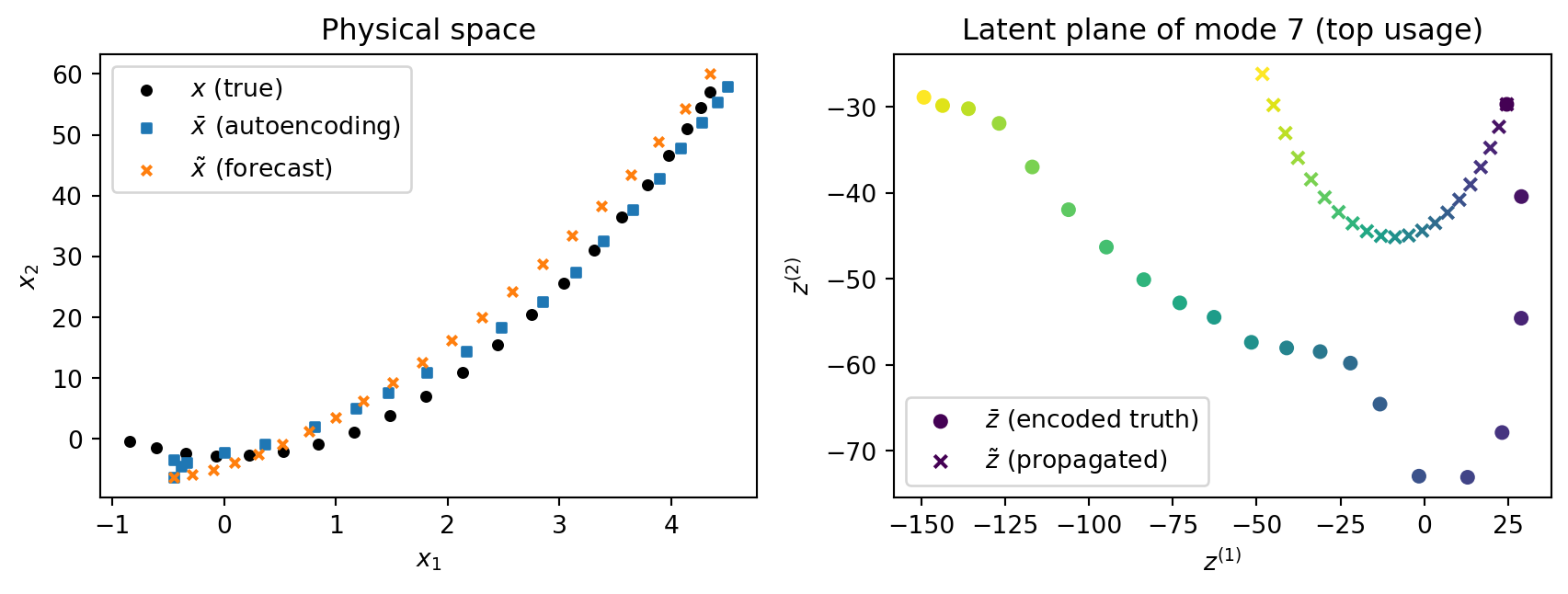
One trajectory first. In the latent plane of the top-usage mode, $\tilde z$ is a logarithmic spiral *by construction* — the question is whether $\bar z$ stays on it.
```{python}
#| label: fig-error-traj
#| fig-cap: "Left: one validation trajectory with its autoencoding $\\bar x$ and its forecast $\\tilde x$. Right: the same trajectory seen in the latent plane of the most used mode — the propagated $\\tilde z$ (crosses) follows an exact logarithmic spiral, the encoded truth $\\bar z$ (dots) should stay on it."
#| code-fold: true
#| code-summary: "Show plotting code"
b0     = 0                    # one validation trajectory
jj_top = usage.argmax()       # most used mode

fig, axs = plt.subplots(1, 2, figsize=(9, 3.5))

axs[0].set_title("Physical space")
axs[0].scatter(*x_val[b0].T, color='k', s=15, label=r"$x$ (true)")
axs[0].scatter(*x_bar[b0].T, color='C0', s=15, marker='s', label=r"$\bar x$ (autoencoding)")
axs[0].scatter(*x_tilde[b0].T, color='C1', s=15, marker='x', label=r"$\tilde x$ (forecast)")
axs[0].set_xlabel(r"$x_1$")
axs[0].set_ylabel(r"$x_2$")
axs[0].legend()

axs[1].set_title(f"Latent plane of mode {jj_top} (top usage)")
axs[1].scatter(*z_bar[b0, :, jj_top].T, c=t_grid, marker='o', s=25, label=r"$\bar z$ (encoded truth)")
axs[1].scatter(*z_tilde[b0, :, jj_top].T, c=t_grid, marker='x', s=25, label=r"$\tilde z$ (propagated)")
axs[1].set_xlabel(r"$z^{(1)}$")
axs[1].set_ylabel(r"$z^{(2)}$")
axs[1].legend()

fig.tight_layout()
plt.show()
```
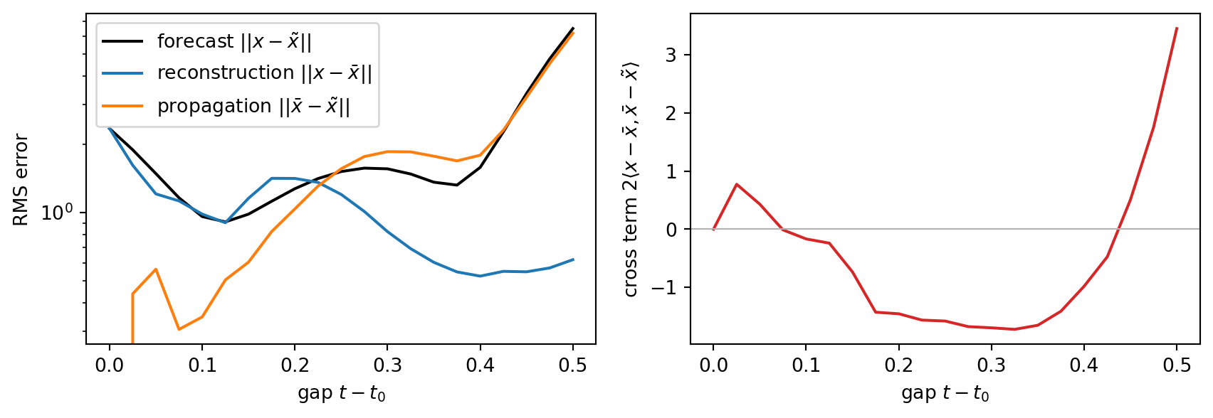
Taking norms in the identity only gives a triangle inequality — the two error vectors can cancel. Squaring restores an exact decomposition:
$$
||x - \tilde x||^2 = ||x - \bar x||^2 + ||\bar x - \tilde x||^2 + 2\,\big\langle x - \bar x,\; \bar x - \tilde x\big\rangle
$$
The cross term measures the cancellation, and is a result in itself:
- clearly negative — co-adaptation: the decoder compensates a bias of the dynamic (nothing supervises the blocks separately)
- negligible — the single unrolling loss kept the blocks honest
This is the trade-off deep Koopman papers address with separate reconstruction and linearity losses.
```{python}
#| label: error-gap
rms   = lambda e: e.norm(dim=-1).pow(2).mean(0).sqrt()          # (k)
cross = 2 * es(e_rec, e_prop, 'b k p, b k p -> b k').mean(0)    # (k)
```
```{python}
#| label: fig-error-gap
#| fig-cap: "Left: RMS of the total error and of its two components as a function of the forecast gap, over the validation set. Right: the cross term of the squared decomposition — negative values indicate cancellation (co-adaptation) between the two error sources."
#| code-fold: true
#| code-summary: "Show plotting code"
fig, axs = plt.subplots(1, 2, figsize=(9, 3.2))

axs[0].plot(t_grid, rms(e_tot), color='k', label=r"forecast $||x - \tilde x||$")
axs[0].plot(t_grid, rms(e_rec), color='C0', label=r"reconstruction $||x - \bar x||$")
axs[0].plot(t_grid, rms(e_prop), color='C1', label=r"propagation $||\bar x - \tilde x||$")
axs[0].set_yscale('log')
axs[0].set_xlabel(r"gap $t - t_0$")
axs[0].set_ylabel("RMS error")
axs[0].legend()

axs[1].plot(t_grid, cross, color='C3')
axs[1].axhline(0, color='0.7', lw=0.8)
axs[1].set_xlabel(r"gap $t - t_0$")
axs[1].set_ylabel(r"cross term $2\langle x - \bar x, \bar x - \tilde x\rangle$")

fig.tight_layout()
plt.show()
```
Reading the curves:
- reconstruction should stay flat — autoencoding does not depend on the horizon
- propagation should grow with the gap
- propagation dominates → improve the dynamic and eigenfunctions; reconstruction dominates → more modes, or the eigenlattice product structure — topic of a follow-up