Matrix Exponential vs Numerical Integration

From Euler steps to exp(At), and how to learn linear dynamics

Forecasting a linear dynamic

Introducing the dynamics

In this tutorial we study the linear ODE

\[\frac{dz}{dt} = Az, \quad z(0) = z_0\]

where \(A \in \mathbb{R}^{2 \times 2}\). The behavior of trajectories is entirely governed by the eigenvalues of \(A\). We illustrate with three canonical cases:

Case	Matrix	Eigenvalues	Behavior
Stable node	\(A_1 = \begin{pmatrix}-2 & 0 \\ 0 & -0.5\end{pmatrix}\)	\(-2,\ -0.5\)	Trajectories collapse to the origin along eigenvector directions
Center	\(A_2 = \begin{pmatrix}0 & -2 \\ 2 & 0\end{pmatrix}\)	\(\pm 2i\)	Closed orbits, energy is conserved
Stable degenerate node	\(A_3 = \begin{pmatrix}-1 & 1 \\ 0 & -1\end{pmatrix}\)	\(-1\) (double)	Converges to origin with a \(t e^{-t}\) transient; non-diagonalizable

import numpy as np
import torch
import matplotlib.pyplot as plt
from torchdiffeq import odeint

A1 = torch.tensor([[-2.0, 0.0],
                   [ 0.0,-0.5]], dtype=torch.float64)   # stable node

A2 = torch.tensor([[ 0.0,-2.0],
                   [ 2.0, 0.0]], dtype=torch.float64)   # center

A3 = torch.tensor([[-1.0, 1.0],
                   [ 0.0,-1.0]], dtype=torch.float64)   # stable degenerate node (Jordan block)

cases = [("Stable node",            A1),
         ("Center",                 A2),
         ("Stable degenerate node", A3)]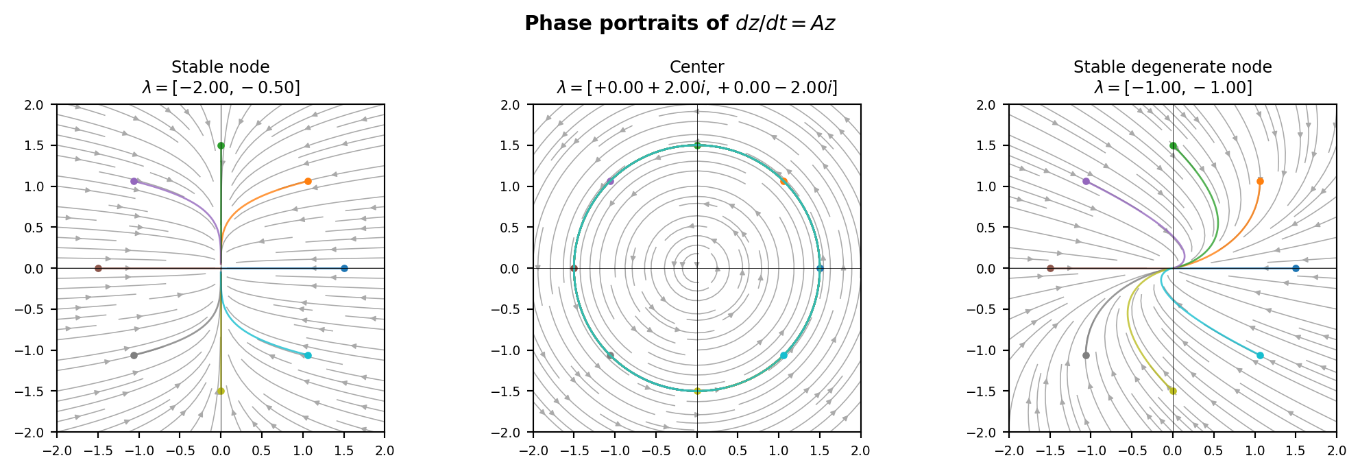

NoteWhy can’t we have one real and one imaginary eigenvalue?

For a real \(2 \times 2\) matrix, the characteristic polynomial is

\[\det(A - \lambda I) = \lambda^2 - \operatorname{tr}(A)\,\lambda + \det(A) = 0\]

with discriminant \(\delta = \operatorname{tr}(A)^2 - 4\det(A)\). The three cases are:

\[\lambda = \frac{\operatorname{tr}(A)}{2} \pm \begin{cases} \frac{1}{2}\sqrt{\delta} & \delta > 0 \quad \text{(two real eigenvalues)} \\ \frac{i}{2}\sqrt{-\delta} & \delta < 0 \quad \text{(complex conjugate pair)} \\ 0 & \delta = 0 \quad \text{(one repeated real eigenvalue)} \end{cases}\]

Complex eigenvalues always come as conjugate pairs \(a \pm bi\), so it is impossible to have one purely real and one purely imaginary eigenvalue for a real matrix.

Link between exponential and numerical integration

We have two ways to propagate a state from \(z_0\) to time \(t\):

\[z(t) = \underbrace{\texttt{odeint}(A,\, z_0,\, t)}_{\text{numerical integration}} \qquad \longleftrightarrow \qquad z(t) = \underbrace{e^{At}\,z_0}_{\text{matrix exponential}}\]

What is the connection between the two? We denote by \(z_e\) the state obtained by the Euler scheme with step size \(\delta_t\):

\[z_e(\delta_t) = z_0 + \delta_t A z_0 = (I + \delta_t A)\,z_0\]

Applying the same step again from \(z_e(\delta_t)\):

\[z_e(2\delta_t) = (I + \delta_t A)\,z_e(\delta_t) = (I + \delta_t A)^2\,z_0 = z_0 + 2\delta_t A z_0 + \delta_t^2 A^2 z_0\]

By induction over \(K\) steps:

\[z_e(K\delta_t) = (I + \delta_t A)^K\,z_0\]

Setting \(t = K\delta_t\) (i.e. \(K = t/\delta_t\)) and taking \(\delta_t \to 0\):

\[z_e(t) = \left(I + \frac{t}{K} A\right)^K z_0 \xrightarrow[K \to \infty]{} e^{At}\,z_0\]

This is exactly the standard limit definition of the matrix exponential. The matrix exponential is the continuous limit of the Euler scheme — accuracy degrades as \(\delta_t\) grows.

z0    = torch.tensor([1.0, 1.5], dtype=torch.float64)
T     = 4.0
t_ref = torch.linspace(0, T, 500, dtype=torch.float64)

# exact solution via matrix exponential for each t
def exact(A, t, z0):
    return (torch.linalg.matrix_exp(A[None] * t[:, None, None]) @ z0).numpy()

# euler with K steps
def euler(A, t_grid, z0):
    return odeint(lambda t, z: A @ z, z0, t_grid, method='euler').numpy()

step_sizes = {f"$\\delta_t={T/10:.2f}$":  torch.linspace(0, T, 10,  dtype=torch.float64),
              f"$\\delta_t={T/50:.2f}$":  torch.linspace(0, T, 50,  dtype=torch.float64),
              f"$\\delta_t={T/500:.3f}$": torch.linspace(0, T, 500, dtype=torch.float64)}
colors_euler = ["#e74c3c", "#e67e22", "#2ecc71"]

fig, axes = plt.subplots(1, 3, figsize=(11, 3.5))
for ax, (title, A) in zip(axes, cases):
    z_ex = exact(A, t_ref, z0)
    ax.plot(z_ex[:,0], z_ex[:,1], 'k-', lw=2, label='exact $e^{At}z_0$')
    for (label, t_grid), color in zip(step_sizes.items(), colors_euler):
        z_eu = euler(A, t_grid, z0)
        ax.plot(z_eu[:,0], z_eu[:,1], '--', color=color, lw=1.2, label=f'Euler {label}')
    ax.plot(*z0.numpy(), 'ko', markersize=5)
    ax.set_title(title, fontsize=9)
    ax.set_xlabel('$z_1$'); ax.set_ylabel('$z_2$')
    ax.set_aspect('equal'); ax.grid(True, alpha=0.3)

axes[0].legend(fontsize=7, loc='best')
fig.suptitle('Euler vs exact $e^{At}z_0$ — three step sizes', fontsize=11, fontweight='bold')
plt.tight_layout()
plt.show()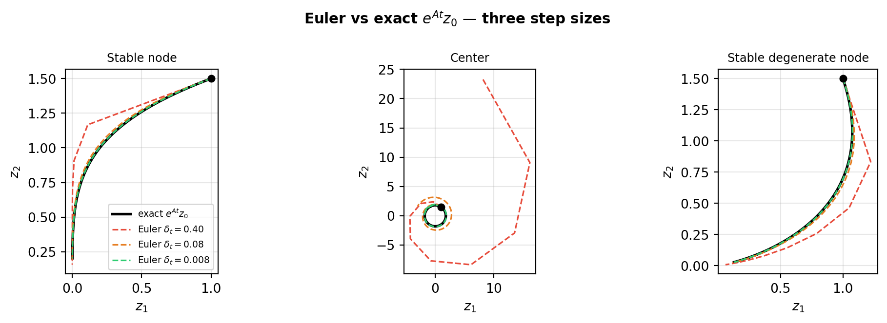

Computation: how to evaluate \(e^{At}z_0\)

Computing \(e^{At}z_0\) is the inner loop of both simulation and learning — every gradient step requires evaluating it, possibly for many values of \(t\) or many initial conditions \(z_0\). The right method depends on three questions:

1. Does cost depend on \(t\)? Some methods pay a fixed upfront cost; others get slower as \(t\) grows.
2. Many \(t\), one \(z_0\)? E.g. predicting a full trajectory from a single initial condition.
3. One \(t\), many \(z_0\)? E.g. a batch of initial conditions all propagated to the same horizon.

We compare four methods on these axes. All code uses a shared setup:

A_ex  = A2
z0_ex = torch.tensor([1.0, 0.5], dtype=torch.float64)
t_ex  = torch.tensor(3.0,        dtype=torch.float64)

Diagonalization

If \(A = VDV^{-1}\), then \(e^{At} = V e^{Dt} V^{-1}\), where \(e^{Dt}\) is cheap to compute (diagonal).

For non-diagonalizable \(A\) this fails; Schur decomposition is the fallback.

L, V = torch.linalg.eig(A_ex)
assert torch.linalg.cond(V) < 1e10, 'Matrix A is not diagonalizable'

# Note that V and L entries are potentially complex, although z_t are real in any way as A is real entry
# Thus to allow computation you need to convert the initial condition to complex and then you can safely convert back to real

z_t  = (V @ torch.diag(torch.exp(L * t_ex)) @ torch.linalg.inv(V) @ z0_ex.cdouble()).real

✓ once you have computed the diagonal form you can evaluate the exponential for free for any \(z_0\) and \(t\)

✗ \(A\) needs to be diagonalizable

Approximate \(e^{At}\)

Approximates \(e^{At}\) as a ratio of matrix polynomials with a scaling-and-squaring step for large \(\|At\|\).

expAt = torch.linalg.matrix_exp(A_ex * t_ex)   # (Apparently what is done in pytorch is similar to Padé)
z_t   = expAt @ z0_ex                            # reuse for any z0

✓ works for any matrix (even non-diagonalizable)

✓ once you have computed \(e^{At}\) you can evaluate \(e^{At}z_0\) for free for any \(z_0\)

✗ need to restart the approximation for every new \(t\)

Approximate \(e^{At}z_0\)

We remember that :

\[ \exp(At)z_0 = \sum_{k=0}^{\infty} \frac{1}{k!} A^k t^k z_0 \]

And that the terms of the sum eventually decay (as \(k\) increases the \(k!\) term dominates \(\|A^k z_0\|_2 \leq \sigma_{\max}^k \|z_0\|_2\))

Thus, rather than forming the full \(n \times n\) matrix \(e^{At}\), we could build a basis as \(\mathcal{K}_m = \text{span}\{z_0,\, Az_0,\, A^2z_0,\,\ldots\}\) of dimension \(m \ll n\) and compute :

\[e^{At}z_0 \approx \sum_{j=0}^{M} \frac{1}{j!} K_j t^j\]

This is the general idea, in practice, the Krylov method builds an orthonormal basis of \(\mathcal{K}_m\) to avoid the numerical instability of summing the raw \(A^j z_0\) terms directly.

PyTorch currently has no built-in function for this, but we can use the one from scipy:

from scipy.sparse.linalg import expm_multiply
z_t = expm_multiply(A_ex.numpy() * t_ex.item(), z0_ex.numpy())

✓ works for any matrix (even non-diagonalizable)

✓ once you have computed the basis you can evaluate \(e^{At}z_0\) for free for any \(t\)

✗ need to rebuild the basis for every new \(z_0\)

Numerical integration (odeint)

Solves \(\dot{z} = Az\) by stepping through intermediate times from \(z_0\) to \(t\). Step size is constrained by the stiffness of \(A\) (ratio of largest to smallest \(|\lambda|\)). Naturally efficient for successive \(t\) values on the same trajectory since all intermediate states are already computed.

z_t    = odeint(lambda t, z: A_ex @ z, z0_ex, torch.tensor([0.0, t_ex]))[-1]

✓ works with \(\dot{z}(t) = A(t) z(t)\) (time-varying linear dynamics)

✓ works for any matrix (even non-diagonalizable), although slow if \(\kappa(A)\) is large

✗ need to restart for every new \(t\) and \(z_0\)

Summary and decision tree

Scenario	Diagonalization	Padé	Krylov	OdeInt
Many \(t\), many \(z_0\)	✓	✗	✗	✗
One \(t\), many \(z_0\)	✓	✓	✗	✗
Many \(t\), one \(z_0\)	✓	✗	✓	✗
Successive \(t\), one \(z_0\)	✓	✗	✗	✓

flowchart LR
    A["dz/dt = A·z"] --> B{"A constant?"}
    B -- No --> C["odeint"]
    B -- Yes --> D{"A large\nand sparse?"}
    D -- Yes --> E{"Many z₀?"}
    E -- Yes --> F["odeint"]
    E -- No  --> G["Krylov"]
    D -- No  --> H{"Many t or z₀?"}
    H -- Yes --> I["Diagonalization"]
    H -- No  --> J["Padé"]