Koopman Complex-Valued Eigenfunctions

A follow-up Q&A on the introduction post

This is a follow-up to Koopman Eigenfunctions — An Introduction. There we kept things simple by working with real-valued eigenfunctions, but in general the Koopman eigenfunctions \(\kpsi_j\), weights \(\kv_j\) and eigenvalues \(\klam_j\) are complex, even when the observable \(\kg\) itself stays real. This note works through why that’s the case, what it costs computationally, and when it actually matters.

In the introduction we wrote

\[ \begin{aligned} x &\in \mathbb{R}^p \\ \kg &: \mathbb{R}^p \to \mathbb{R} \quad \text{(observation function)} \\ \kg(x) &= \sum_{j=0}^{\infty} \kv_j \kpsi_j(x) \end{aligned} \]

Where

\[ \begin{aligned} \kpsi_j(T(x_0, t)) &= e^{\klam_j t}\kpsi_j(x_0) \end{aligned} \]

Here \(\kv_j\) are the weights in the decomposition, \(\kpsi_j\) are the eigenfunctions of the dynamic and \(\klam_j\) their associated eigenvalues.

Question 1: can the eigenspace be complex?

In practice it would mean \(\kpsi_j: \mathbb{R}^p \to \mathbb{C}\), \(\kv_j \in \mathbb{C}\), \(\klam_j \in \mathbb{C}\).

At first sight it can seem surprising as \(\kg(x) \in \mathbb{R}\) and \(\kg(x) = \sum_{j=0}^{\infty} \kv_j \kpsi_j(x)\), summing complex numbers is going to return a complex number.

But if the dynamic in Koopman space were operating on real numbers only, it would restrict the ability to represent oscillations, for instance.

Response

Actually, Koopman eigenfunctions can be complex. The idea is that they always come in conjugate pairs \((\kpsi_j, \overline{\kpsi_j})\), and for any real observable \(\kg\) the corresponding coefficients must themselves be complex conjugates of each other, in this way:

\[ \kg(x) = \sum_{j=0}^{\infty} \kv_j \kpsi_j(x) = \sum_{\text{pairs}\ j} \left( \kv_j \kpsi_j(x) + \overline{\kv_j}\, \overline{\kpsi_j(x)} \right) = 2 \sum_{\text{pairs}\ j} \mathrm{Re}\big(\kv_j \kpsi_j(x)\big) \]

where the last two sums run over one representative of each conjugate pair (an eigenfunction with a real eigenvalue can be taken real and enters the sum directly, without the factor 2). Thus \(\kg(x)\) stays real while the \(\kpsi_j\) themselves are complex.

NoteProposition

Let \(\kpsi_j\) be a Koopman eigenfunction of \(T\) with eigenvalue \(\klam_j \in \mathbb{C}\). Then \(\overline{\kpsi_j}\) is also a Koopman eigenfunction of \(T\), with eigenvalue \(\overline{\klam_j}\).

TipProof

Let \(\kpsi_k \triangleq \overline{\kpsi_j}\), i.e. \(\kpsi_k(x) = \overline{\kpsi_j(x)} \; \forall x\), and write \(x_t = T(x_0, t)\). Thus:

\[ \begin{aligned} \kpsi_k(x_t) &= \overline{\kpsi_j(x_t)}\\ &= \overline{e^{\klam_j t}\kpsi_j(x_0)}\\ &= e^{\overline{\klam_j} t}\, \overline{\kpsi_j(x_0)}\\ &= e^{\overline{\klam_j} t}\, \kpsi_k(x_0) \quad \forall x_0, t \end{aligned} \]

so \(\kpsi_k\) satisfies the eigenfunction relation with eigenvalue \(\overline{\klam_j}\).

Question 2: if we keep only the \(\mathrm{Re}(\kpsi_j(x))\) do we still need to do integration on complex numbers?

Yes, because the imaginary parts of \(\klam_j\) and \(\kpsi_j(x_0)\) are going to impact \(\mathrm{Re}(\kpsi_j(x))\). Writing \(\klam_j = \gamma + \omega i\):

\[ e^{\klam_j t}\,\kpsi_j(x) = e^{(\gamma+\omega i)t}\big(a_j(x)+ib_j(x)\big) = e^{(\gamma+\omega i)t}\, r_j(x)\, e^{i\varphi_j(x)} \]

with \(r_j(x) = \sqrt{a_j(x)^2 + b_j(x)^2}\) and \(\varphi_j(x) = \operatorname{atan2}\big(b_j(x),\, a_j(x)\big)\)

Thus:

\[ e^{\klam_j t}\,\kpsi_j(x) = r_j(x)\, e^{\gamma t + i(\omega t + \varphi_j(x))} = r_j(x)\, e^{\gamma t}\Big(\cos(\omega t+\varphi_j(x)) + i\sin(\omega t+\varphi_j(x))\Big) \]

Thus \(\mathrm{Re}(e^{\klam_j t}\,\kpsi_j(x)) = r_j(x)\, e^{\gamma t}\cos(\omega t+\varphi_j(x))\), we can see the real part is impacted by \(\omega\) and \(b_j\) (the imaginary parts of the eigenvalue and initial condition).

Question 3: for what kind of dynamic do we need complex eigenfunctions?

If we take a simple dynamic like:

\[ \frac{dx}{dt} = Ax \]

With \(x \in \mathbb{R}^p\) and \(A \in \mathbb{R}^{p \times p}\), we can show that \(\kpsi_j(x) = l_j \cdot x\) are Koopman eigenfunctions, where \(l_j A = \klam_j l_j\) are the left eigenvectors of \(A\):

\[ \kpsi_j(T(x_0, t)) = \kpsi_j(e^{At}x_0) = l_j \cdot e^{At} x_0 = e^{\klam_j t}\, l_j \cdot x_0 = e^{\klam_j t} \kpsi_j(x_0) \]

using \(l_j\, e^{At} = e^{\klam_j t}\, l_j\), which follows from applying \(l_j A = \klam_j l_j\) term by term in the series \(e^{At} = \sum_n \frac{(At)^n}{n!}\).

Thus, if some left eigenvectors of \(A\) (and their corresponding eigenvalues) are complex, the resulting eigenfunctions will be complex too.

Example

Take \(A\) to be a pure rotation generator in \(\mathbb{R}^2\), with state \(x = (x_1, x_2)\) (drawn as \((x,y)\) in the board sketch at the end of this post):

\[ \dot{x} = Ax, \qquad A = \begin{bmatrix} 0 & -\omega \\ \omega & 0 \end{bmatrix} \]

Koopman eigenfunctions:

\(A\) has two complex left eigenvectors, conjugate of each other as expected from the Proposition above:

\[ \begin{aligned} l_1 &= \begin{bmatrix} 1 & i \end{bmatrix}, & \klam_1 &= i\omega \\ l_2 &= \begin{bmatrix} 1 & -i \end{bmatrix} = \overline{l_1}, & \klam_2 &= -i\omega = \overline{\klam_1} \end{aligned} \]

giving the two conjugate eigenfunctions:

\[ \kpsi_1(x) = l_1 \cdot x = x_1 + i x_2, \qquad \kpsi_2(x) = l_2 \cdot x = x_1 - i x_2 = \overline{\kpsi_1(x)} \]

each evolving as a pure phasor:

\[ \kpsi_1(T(x_0,t)) = e^{i\omega t}\kpsi_1(x_0), \qquad \kpsi_2(T(x_0,t)) = e^{-i\omega t}\kpsi_2(x_0) \]

i.e. \(\kpsi_1\) rotates at rate \(\omega\) and \(\kpsi_2\) at rate \(-\omega\) in \(\mathbb{C}\), while \(x\) itself rotates in the physical plane — reproducing the two circular sketches from the board photo at the end of this post:

import numpy as np
from scipy.linalg import expm
import matplotlib.pyplot as plt

omega = 1.0
A = np.array([[0, -omega],
              [omega, 0]])
x0 = np.array([1.0, 0.3])              # initial condition

t = np.linspace(0, 0.3, 200)           # only the start of the trajectory

# physical-space trajectory: x(t) = e^{At} x0
x_t = np.array([expm(A * ti) @ x0 for ti in t])

# eigenfunctions: psi_1(x) = l1 . x, psi_2(x) = l2 . x
l1 = np.array([1, 1j])
l2 = np.array([1, -1j])
psi1 = x_t @ l1
psi2 = x_t @ l2

lambda1, lambda2 = 1j * omega, -1j * omega
arrow_len = 0.15

fig, axes = plt.subplots(1, 2, figsize=(10, 4.5))

ax = axes[0]
ax.plot(x_t[:, 0], x_t[:, 1], color="tab:red")
ax.scatter([x0[0]], [x0[1]], color="tab:red", zorder=5)
ax.annotate(r"$x(0)$", xy=(x0[0], x0[1]), xytext=(5, 5), textcoords="offset points", color="tab:red")
v_phys = A @ x_t[-1]                                   # dx/dt = A x, at the endpoint
v_phys = v_phys / np.linalg.norm(v_phys) * arrow_len
ax.annotate("", xy=x_t[-1] + v_phys, xytext=x_t[-1],
            arrowprops=dict(arrowstyle="-|>", color="tab:red", lw=1.5))
A_label = "A = ⎡ 0   -ω ⎤\n    ⎣ ω    0 ⎦"
ax.annotate(A_label, xy=x_t[-1] + v_phys, xytext=(6, 6), textcoords="offset points",
            color="tab:red", fontsize=9, family="monospace")
ax.axhline(0, color="black", lw=0.8)
ax.axvline(0, color="black", lw=0.8)
ax.set_xlabel(r"$x_1$")
ax.set_ylabel(r"$x_2$")
ax.set_title("Physical space")
ax.set_xlim(-1.2, 1.2)
ax.set_ylim(-1.2, 1.2)
ax.set_aspect("equal")

ax = axes[1]
c1, c2 = plt.cm.viridis(0.15), plt.cm.viridis(0.85)    # viridis colors for psi_1, psi_2
ax.plot(psi1.real, psi1.imag, color=c1)
ax.plot(psi2.real, psi2.imag, color=c2)
ax.scatter([psi1[0].real], [psi1[0].imag], color=c1, zorder=5)
ax.scatter([psi2[0].real], [psi2[0].imag], color=c2, zorder=5)
ax.annotate(r"$\psi_1(x_0)$", xy=(psi1[0].real, psi1[0].imag), xytext=(5, 5), textcoords="offset points", color=c1)
ax.annotate(r"$\psi_2(x_0)$", xy=(psi2[0].real, psi2[0].imag), xytext=(5, 5), textcoords="offset points", color=c2)
arrow_specs = [(psi1[-1], lambda1, c1, r"$\lambda_1$", (6, 6)),
               (psi2[-1], lambda2, c2, r"$\lambda_2$", (14, 6))]
for psi_end, lam, color, lam_label, label_offset in arrow_specs:
    v = lam * psi_end                                  # dpsi/dt = lambda psi, at the endpoint
    v = v / abs(v) * arrow_len
    end = psi_end + v
    ax.annotate("", xy=(end.real, end.imag), xytext=(psi_end.real, psi_end.imag),
                arrowprops=dict(arrowstyle="-|>", color=color, lw=1.5))
    ax.annotate(lam_label, xy=(end.real, end.imag), xytext=label_offset,
                textcoords="offset points", color=color)
ax.axhline(0, color="black", lw=0.8)
ax.axvline(0, color="black", lw=0.8)
ax.set_xlabel("Re")
ax.set_ylabel("Im")
ax.set_title("Koopman space")
ax.set_xlim(-1.2, 1.2)
ax.set_ylim(-1.2, 1.2)
ax.set_aspect("equal")

plt.tight_layout()
plt.show()

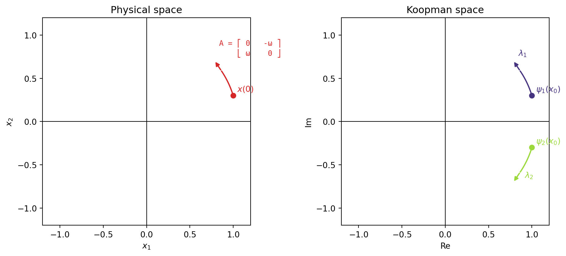
Figure 1: Physical-space trajectory (left) and the two conjugate eigenfunctions \(\psi_1\), \(\psi_2\) as counter-rotating phasors in the complex plane (right).

NoteEigenfunction products form a lattice

Products of eigenfunctions are eigenfunctions too, with summed eigenvalues:

\[ \big(\kpsi_1 \kpsi_2\big)(T(x,t)) = \kpsi_1(T(x,t))\,\kpsi_2(T(x,t)) = e^{(\klam_1+\klam_2) t}\,\kpsi_1(x)\,\kpsi_2(x) \]

Here \(\klam_1+\klam_2 = 0\), and indeed \(\kpsi_1(x)\kpsi_2(x) = x_1^2+x_2^2 = \lVert x \rVert^2\), the squared radius — a conserved quantity under a pure rotation, consistent with eigenvalue \(0\).

Reconstruction:

Decomposition of the coordinate observables \(\kg_1(x) = x_1\) and \(\kg_2(x) = x_2\) in the \(\{\kpsi_1,\kpsi_2\}\) basis, using \(\kv_2 = \overline{\kv_1}\) each time (per the Proposition above):

\[ \begin{aligned} \kg_1(x) = x_1 &= \tfrac{1}{2}\kpsi_1(x) + \tfrac{1}{2}\kpsi_2(x) & (\kv_1 = \tfrac12 \text{ real}) \\ \kg_2(x) = x_2 &= -\tfrac{i}{2}\kpsi_1(x) + \tfrac{i}{2}\kpsi_2(x) & (\kv_1 = -\tfrac{i}{2} \text{ purely imaginary}) \end{aligned} \]

Conclusion

Koopman eigenfunctions of a dynamic in real space can be complex and it’s important to represent them in that way. In some works a neural network (encoder) is used to represent Koopman eigenfunctions. In deep learning frameworks it is not common for networks to take real-valued inputs and output complex numbers, so one has to be extra careful about that.

NoteBoard sketch

Sometimes it’s more intuitive to look at the board: