Representation learning for action-angle coordinates

Author

Etienne Meunier

Published

November 3, 2026

In this post we show that we can learn the invariant of a dynamic from trajectories alone; those invariants are then useful to infer and learn the dynamic itself. We start with a pendulum and simulate a few trajectories.

Show imports

import torch
import torch.nn as nn
import torch.func as F
import einops
import numpy as np
import matplotlib.pyplot as plt
from torchdiffeq import odeint

1 Simulating data

We start by simulating a few pendulum trajectories at different energy levels. \[ \ddot\theta = -\sin\theta \qquad\Longrightarrow\qquad \begin{cases} \dot\theta = \omega \\ \dot\omega = -\sin\theta \end{cases} \] \[ \kH(\theta, \dot\theta) = \tfrac{1}{2}\dot\theta^2 + 1 - \cos\theta \]

Code

def pendulum_dyn(t, state):
    return torch.stack([state[..., 1], -torch.sin(state[..., 0])], dim=-1)

def hamiltonian(state):
    return 0.5 * state[..., 1] ** 2 + 1 - torch.cos(state[..., 0])

def init_cond(H):
    """theta at rest (thetadot=0) for a given energy H."""
    return torch.arccos(1 - H)

t = torch.linspace(0, 20, 100)
init_theta = init_cond(torch.linspace(0, 2, 10))
init_x = torch.stack([init_theta, torch.zeros_like(init_theta)], dim=-1)

training_set = odeint(pendulum_dyn, init_x, t)
t_exp = t[:, None, None].expand(*training_set.shape[:-1], 1)
training_set = torch.cat([t_exp, training_set], dim=-1)
training_set = einops.rearrange(training_set, 't h c -> h t c')   # (level, time, [t, theta, thetadot])

Show plotting code

colors = plt.get_cmap('viridis')(np.linspace(0.1, 0.9, training_set.shape[0]))

fig, ax = plt.subplots(figsize=(5, 5))
for i in range(training_set.shape[0]):
    ax.plot(training_set[i, :, 1], training_set[i, :, 2], color=colors[i])
ax.set(xlabel=r'$\theta$', ylabel=r'$\dot\theta$', title='training trajectories', xlim=(-3, 3), ylim=(-3, 3))
plt.show()

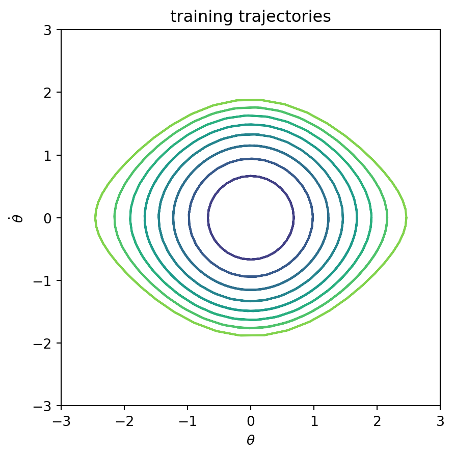
Figure 1: Ten pendulum trajectories released from rest at different energies.

We know that the energy $\kH$ is conserved along each trajectory — an invariant — and takes a different value for each trajectory, since they start at different points. That’s exactly the structure we are going to exploit here.

2 Learning an invariant

Our goal is to learn a representation $\kE(\text{state})$ that is the same along a trajectory but different between trajectories — that’s simply what we train the model for:

Let $x_{i,t} \sim \mathcal D$ denote the state at time $t$ on trajectory $i$: \[ \mathcal L = \log\Big(\underbrace{\mathbb E_i\big[\mathrm{Var}_t(\kE(x_{i,t}))\big]}_{\text{consistency}}\Big) - \log\Big(\underbrace{\mathrm{Var}_i\big[\mathbb E_t(\kE(x_{i,t}))\big]}_{\text{diversity}}\Big) \]

Code

def loss_f(preds):
    diversity = preds.mean(dim=1).var()     # variance over trajectories
    consistency = preds.var(dim=1).mean()   # variance over time
    loss = torch.log(consistency) - torch.log(diversity)
    return loss

There is no restriction on the network we want to train, except that it is a smooth $\mathbb R^p \to \mathbb R$ function.

Code

class Encoder(nn.Module):
    """(theta, thetadot) -> I, a simple 2 -> 1 MLP."""

    def __init__(self, hidden=64, n_layers=3):
        super().__init__()
        layers = [nn.Linear(2, hidden), nn.Tanh()]
        for _ in range(n_layers - 1):
            layers += [nn.Linear(hidden, hidden), nn.Tanh()]
        layers += [nn.Linear(hidden, 1)]
        self.net = nn.Sequential(*layers)

    def forward(self, x):
        return self.net(x).squeeze(-1)

encoder = Encoder()

We just train by taking batches of trajectories and minimizing the representation loss.

Code

optimizer = torch.optim.LBFGS(encoder.parameters(), lr=1.0, max_iter=20, line_search_fn="strong_wolfe")
n_epochs = 100   # each step() already runs up to max_iter internal iterations

def closure():
    optimizer.zero_grad()
    I = encoder(training_set[..., 1:])   # (n_levels, n_times)
    loss = loss_f(I)
    loss.backward()
    return loss

for epoch in range(n_epochs):
    loss = optimizer.step(closure)
    if epoch % 20 == 0:
        print(f"epoch {epoch:4d}  loss {loss.item(): .4e}")

epoch    0  loss  4.1097e+00
epoch   20  loss -1.2861e+01
epoch   40  loss -1.3517e+01
epoch   60  loss -1.3517e+01
epoch   80  loss -1.3517e+01

And now we can visualize the output of the network on our phase space, next to the Hamiltonian.

Show plotting code

g_theta = torch.linspace(-torch.pi, torch.pi, 100)
g_thetadot = torch.linspace(-3, 3, 100)
grid = torch.stack(torch.meshgrid([g_theta, g_thetadot], indexing='xy'), dim=-1)

g_H = hamiltonian(grid)
g_H[g_H > 2] = torch.nan
g_E = encoder(grid).detach()
g_E[hamiltonian(grid) > 2] = torch.nan

fig, axs = plt.subplots(1, 2, figsize=(11, 4.5))
for a, field, title in zip(axs, [g_H, g_E], ['Hamiltonian $H(x)$', 'encoder(x)']):
    cf = a.contourf(g_theta, g_thetadot, field)
    fig.colorbar(cf, ax=a)
    a.set(title=title, xlabel=r'$\theta$', ylabel=r'$\dot\theta$', xlim=(-3, 3), ylim=(-3, 3))
fig.tight_layout()
plt.show()

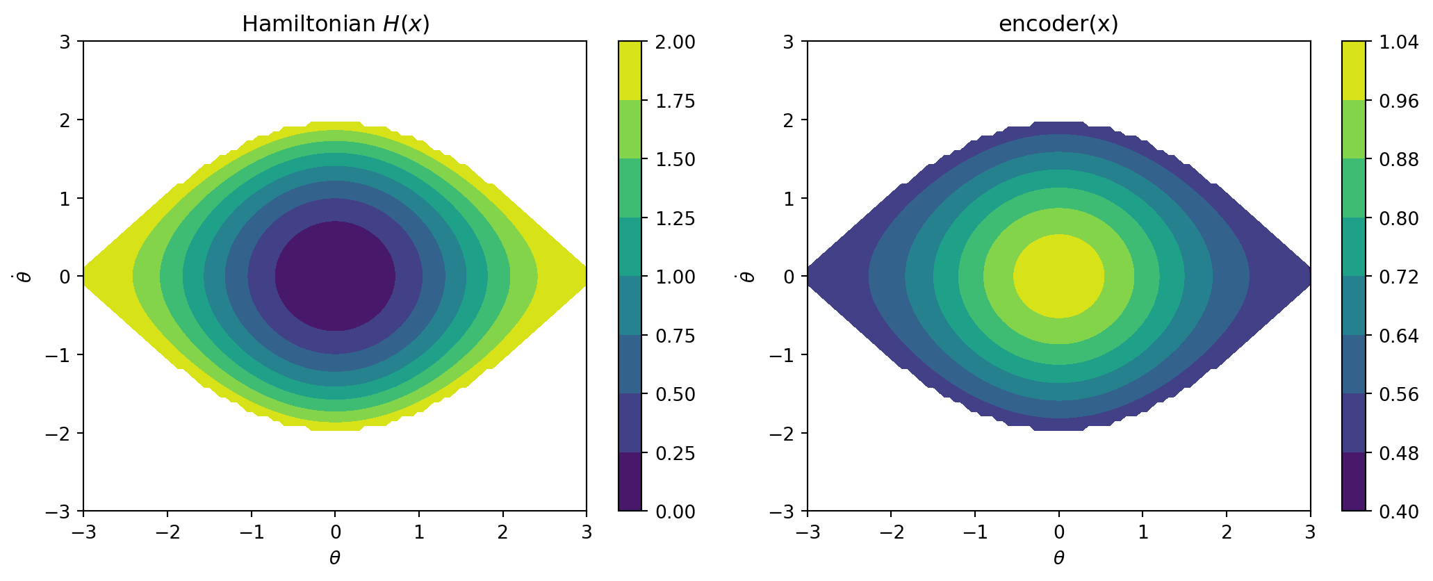
Figure 2: The Hamiltonian (left) vs. the trained encoder (right), over the phase space.

They are quite different — although they share a characteristic: both are smooth functions, monotonically decreasing outward from the fixed point, and since they are both constant on real trajectories they share something even better: contour lines.

Show plotting code

fig, axs = plt.subplots(1, 2, figsize=(11, 4.5))
for a, field, title in zip(axs, [g_H, g_E], ['Hamiltonian $H(x)$', 'encoder(x)']):
    a.contour(g_theta, g_thetadot, field, colors='k', linewidths=0.8)
    a.set(title=title, xlabel=r'$\theta$', ylabel=r'$\dot\theta$', xlim=(-3, 3), ylim=(-3, 3))
fig.tight_layout()
plt.show()

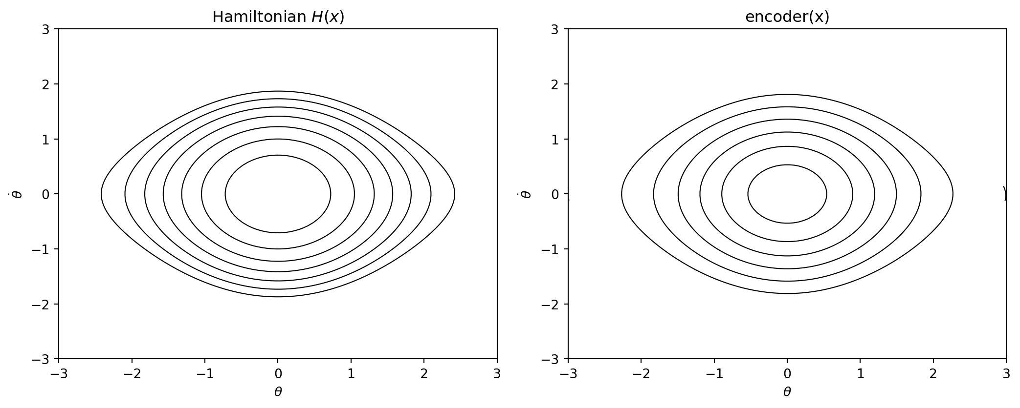
Figure 3: Level sets of the Hamiltonian (left) vs. the trained encoder (right) — same shape, arbitrary scale.

3 Dynamics from the contour lines

From the contour lines we can retrieve the direction of the dynamics at each point: $\kH(x(t))$ is constant $\forall t$, so \[ \frac{d\kH(x)}{dt} = 0 \;\to\; \nabla \kH(x) \cdot \frac{dx}{dt} = 0 \;\to\; \frac{dx}{dt} = \kalpha(x) \nabla^{\perp} \kH(x) \] so the dynamics must be a scaling $\kalpha(x)$ of the perp gradient along the contour line, where \[ \nabla^{\perp} \kH(x) = \begin{bmatrix}0 & 1 \\ -1 & 0\end{bmatrix} \nabla \kH(x) \] We can already draw a stream plot of the dynamic, taking $\kalpha(x) = 1$ for now.

Show plotting code

def perp(g):
    return torch.stack([g[..., 1], -g[..., 0]], dim=-1)

grid_req = grid.clone().requires_grad_(True)
grad_E = torch.autograd.grad(hamiltonian(grid_req).sum(), grid_req)[0]

grid_req = grid.clone().requires_grad_(True)
grad_enc = torch.autograd.grad(encoder(grid_req).sum(), grid_req)[0]

mask = (hamiltonian(grid) > 2).float()
pend_vel = torch.stack([grid[..., 1], -torch.sin(grid[..., 0])], dim=-1)

fig, axs = plt.subplots(1, 3, figsize=(16, 5))
titles = ['pendulum dynamics', r'$\nabla^\perp H$', r'$\nabla^\perp$ encoder']
fields = [pend_vel, perp(grad_E), perp(grad_enc)]
for a, title, field in zip(axs, titles, fields):
    a.streamplot(g_theta.numpy(), g_thetadot.numpy(), field[..., 0].detach().numpy(), field[..., 1].detach().numpy())
    a.contourf(g_theta.numpy(), g_thetadot.numpy(), mask.numpy(), levels=[0.5, 1.5], colors=['lightblue'], alpha=0.5)
    a.set(title=title, xlabel=r'$\theta$', ylabel=r'$\dot\theta$', xlim=(-3, 3), ylim=(-3, 3))
fig.tight_layout()
plt.show()

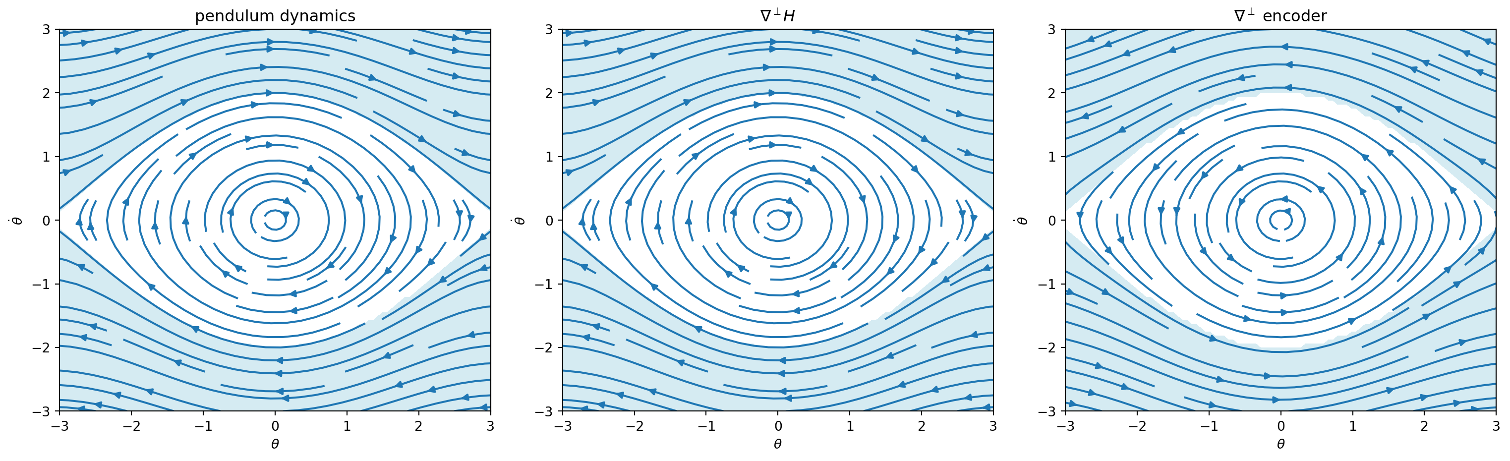
Figure 4: Pendulum dynamics (left) vs. $\nabla^\perp \kH$ (middle) vs. $\nabla^\perp\text{encoder}$ (right). Librium region shaded.

They are following the same lines! Let’s go for the integration.

Show plotting code

grad_hamiltonian_fn = F.grad(hamiltonian)
grad_encoder_fn = F.grad(encoder)

def hamiltonian_dyn(t, state):
    return perp(grad_hamiltonian_fn(state))

def encoder_dyn(t, state):
    return perp(grad_encoder_fn(state))

x0 = torch.tensor([1.0, 0.5])
t_traj = torch.linspace(0, 2, 1000)

traj_pend = odeint(pendulum_dyn, x0, t_traj)
traj_hamiltonian = odeint(hamiltonian_dyn, x0, t_traj)
traj_enc = odeint(encoder_dyn, x0, t_traj)

fig, axs = plt.subplots(1, 3, figsize=(16, 5))
for a, traj, title in zip(axs, [traj_pend, traj_hamiltonian, traj_enc], ['pendulum', r'$\nabla^\perp H$', r'$\nabla^\perp$ encoder']):
    a.plot(traj[:, 0].detach(), traj[:, 1].detach())
    a.plot(x0[0], x0[1], 'ro', ms=8)
    a.set(title=title, xlabel=r'$\theta$', ylabel=r'$\dot\theta$', xlim=(-3, 3), ylim=(-3, 3))
fig.tight_layout()
plt.show()

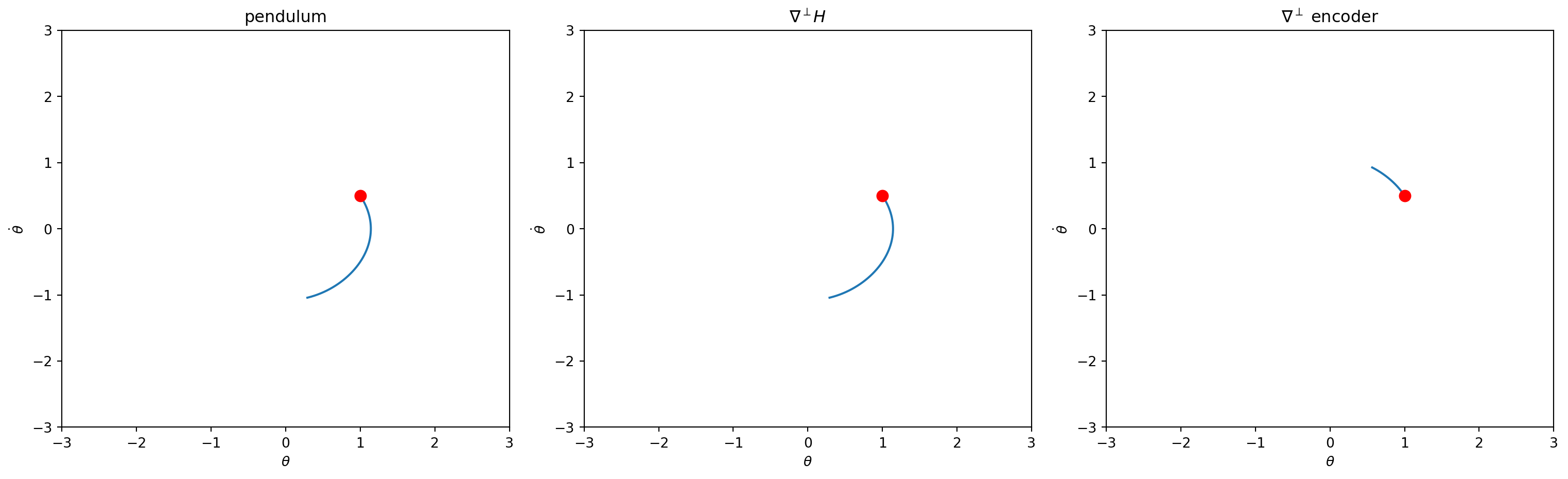
Figure 5: Integrating $\dot x = \nabla^\perp \kH(x)$ and $\dot x = \nabla^\perp \text{encoder}(x)$ from the same $x_0$: right shape, wrong speed.

We can see they are on the same orbit, great — but they don’t have the same speed! So far we took $\kalpha(x) = 1$, an arbitrary scaling of the velocity. To get a proper integration we have to calibrate it.

4 Calibrating

As mentioned above, we can get the direction of the dynamic from the gradient of the invariant, but we still have to learn its velocity — that’s what we do in this section.

In a data-driven framework this step makes a lot of sense: so far we have only exploited the state information $(\theta_i, \dot\theta_i)$, not the associated time $t_i$. We need to include it in the training to learn the velocity.

Our dynamic then takes this form, where $\kc : \mathbb R^p \to \mathbb R$ is the function we want to learn: \[ f_{\theta}(x) = \kc(x) \nabla^{\perp} \kE(x) \]

\[ \theta^* = \underbrace{\arg \min_\theta \int_{x \in \mathbb R^p}||f(x) - f_\theta(x)||dx}_{\text{Offline}} \Longleftrightarrow \theta^* = \underbrace{\arg \min_\theta \sum_{(t_i, x_i) \in \mathcal D}||\Phi(t_i, f, x_i) - \Phi(t_i, f_\theta, x_i)||}_{\text{Online}} \]

Tip

You can only use the offline objective if you have access to the true dynamic; the online one only requires observations and their associated times.

4.1 Hypothesis on the form of $\kc$

Now that we have our learning framework, we can make hypotheses on the form of $\kc$, which impacts the way we learn it:

\[ \kc(x) \to \kc(\kE(x)) \to \kc \]

From left to right, $\kc(x)$ depends on the full state, then we hypothesize one $\kc$ per “level of invariant”, then a single common $\kc$ for the full dynamic.

What makes sense in the pendulum case?

In the case of the pendulum we know there exists a Hamiltonian such that: \[ \frac{dx}{dt} = \nabla^{\perp}\kH(x) \] As $\kH(x)$ and $\kE(x)$ share the same level sets (they are both constant on the trajectories) we can show that $\kH(x) = g(\kE(x))$ where $g$ is a smooth function, then $\nabla \kH(x)= g'(\kE(x)) \nabla \kE(x)$. Thus $\kc$ only needs to depend on $\kE(x)$.

We can implement $\kc$ as a small network taking the invariant value and returning a velocity:

Code

class Speed(nn.Module):
    """I -> scalar calibration factor c(I), s.t. perp(grad I) * c(I) matches true speed."""

    def __init__(self, hidden=32):
        super().__init__()
        self.net = nn.Sequential(
            nn.Linear(1, hidden), nn.Tanh(),
            nn.Linear(hidden, hidden), nn.Tanh(),
            nn.Linear(hidden, 1),
        )

    def forward(self, I):
        return self.net(I.unsqueeze(-1)).squeeze(-1)

for p in encoder.parameters():
    p.requires_grad_(False)
encoder.eval()

speed = Speed()

def calibrated_dyn(x0):
    """Returns dx/dt = c * perp(grad E(x)), with c = c_theta(E(x0)) fixed for the whole rollout —
    E(x0) is conserved along the trajectory, so c is constant by construction, not re-derived at each x."""
    c = speed(encoder(x0))   # x0 is batched: (n, 2)

    def dyn(_, x):
        grad_I = F.vmap(grad_encoder_fn)(x)
        return perp(grad_I) * c.unsqueeze(-1)

    return dyn

4.2 Learning $\kc(\kE)$?

Now we can train Speed very simply:

Training recipe

Take a pair of points from the same trajectory ($x_{t_1}$, $x_{t_2}$)
Compute $c = \kc(\kE(x_{t_1}))$ from our model
Integrate from $x_{t_1}$ for $(t_2 - t_1)$ time with dynamic $f_\theta(x) = c\, \nabla^{\perp} \kE(x)$
Backpropagate the loss through the integration

During this process $\kE$ is frozen: we only train the velocity network, not the invariant.

Code

dt = (training_set[0, 1, 0] - training_set[0, 0, 0]).item()
x0_pairs = training_set[:, :-1, 1:].reshape(-1, 2)   # (n_levels * (n_t - 1), 2)
x1_pairs = training_set[:, 1:, 1:].reshape(-1, 2)

def rollout(x0, dt):
    sol = odeint(calibrated_dyn(x0), x0, torch.tensor([0.0, dt]))
    return sol[-1]

speed_optimizer = torch.optim.LBFGS(speed.parameters(), lr=1.0, max_iter=20, line_search_fn="strong_wolfe")
n_epochs = 50   # each step() already runs up to max_iter internal iterations

def speed_closure():
    speed_optimizer.zero_grad()
    x1_hat = rollout(x0_pairs, dt)
    loss = (x1_hat - x1_pairs).pow(2).mean()
    loss.backward()
    return loss

for epoch in range(n_epochs):
    loss = speed_optimizer.step(speed_closure)
    if epoch % 10 == 0:
        print(f"epoch {epoch:4d}  loss {loss.item(): .4e}")

epoch    0  loss  2.2420e-02
epoch   10  loss  1.6407e-06
epoch   20  loss  1.6407e-06
epoch   30  loss  1.6407e-06
epoch   40  loss  1.6407e-06

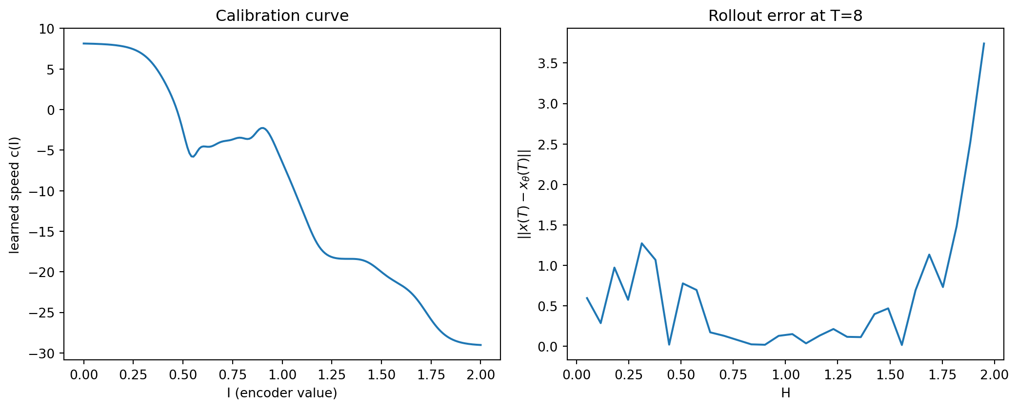
Now that training is done, we can visualize our “calibration curve”: the velocity we associate to each invariant level. We can also check how well it generalizes by rolling out both dynamics to a fixed $T$ (long enough to cover a full period at any energy level) and measuring $||x(T) - x_\theta(T)||$ across the energy range.

Show plotting code

I_grid = torch.linspace(0.0, 2.0, 200)
c_grid = speed(I_grid).detach()

H_levels = torch.linspace(0.05, 1.95, 30)
starts_err = torch.stack([init_cond(H_levels), torch.zeros_like(H_levels)], dim=-1)

T = 8.0
true_T = odeint(pendulum_dyn, starts_err, torch.tensor([0.0, T]))[-1]
calib_T = odeint(calibrated_dyn(starts_err), starts_err, torch.tensor([0.0, T]))[-1]
err = (true_T - calib_T).norm(dim=-1).detach()

fig, axs = plt.subplots(1, 2, figsize=(11, 4.5))
axs[0].plot(I_grid, c_grid)
axs[0].set(xlabel='I (encoder value)', ylabel='learned speed c(I)', title='Calibration curve')
axs[1].plot(H_levels, err)
axs[1].set(xlabel='H', ylabel=r'$||x(T) - x_\theta(T)||$', title=f'Rollout error at T={T:.0f}')
fig.tight_layout()
plt.show()

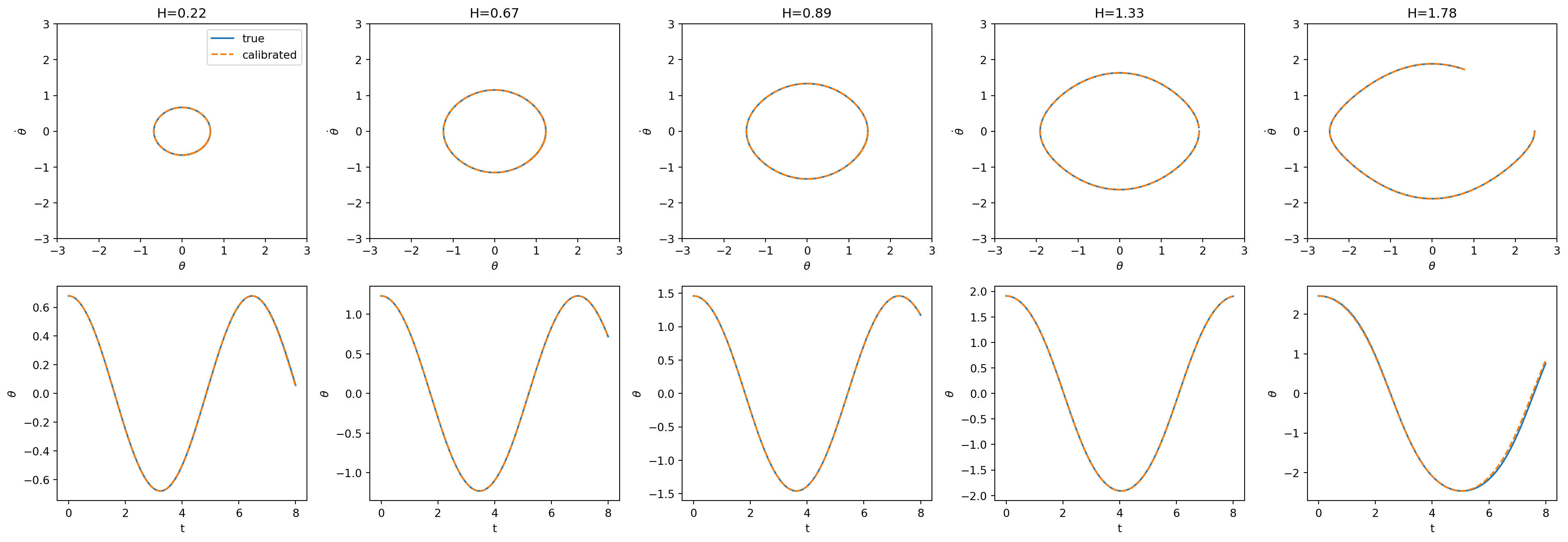
Figure 6: Calibration curve $c(I)$ (left) and rollout error $||x(T) - x_\theta(T)||$ at $T=8$ across energy levels (right).

And try integrating with our newly learned dynamic:

Show plotting code

n_samples = 5
levels = torch.linspace(1, 8, n_samples).round().long()   # skip H=0 (fixed point) and H=2 (separatrix)
starts = training_set[levels, 0, 1:]

t_eval = torch.linspace(0, 8, 300)
true_traj = odeint(pendulum_dyn, starts, t_eval)
calib_traj = odeint(calibrated_dyn(starts), starts, t_eval)

fig, axs = plt.subplots(2, n_samples, figsize=(4 * n_samples, 7))
for i in range(n_samples):
    H_i = hamiltonian(starts[i]).item()

    ax = axs[0, i]
    ax.plot(true_traj[:, i, 0].detach(), true_traj[:, i, 1].detach(), label='true')
    ax.plot(calib_traj[:, i, 0].detach(), calib_traj[:, i, 1].detach(), '--', label='calibrated')
    ax.set(title=f'H={H_i:.2f}', xlabel=r'$\theta$', ylabel=r'$\dot\theta$', xlim=(-3, 3), ylim=(-3, 3))
    if i == 0:
        ax.legend()

    ax = axs[1, i]
    ax.plot(t_eval, true_traj[:, i, 0].detach(), label='true')
    ax.plot(t_eval, calib_traj[:, i, 0].detach(), '--', label='calibrated')
    ax.set(xlabel='t', ylabel=r'$\theta$')

fig.tight_layout()
plt.show()

Figure 7: True vs. calibrated dynamics at five energy levels — phase portrait (top), $\theta(t)$ (bottom).

--- title: "Representation learning for action-angle coordinates" author: "Etienne Meunier" date: today format: html: number-sections: true code-fold: show code-tools: true include-in-header: text: | <script> window.MathJax = { tex: { macros: { kH: ["\\textcolor{#d62728}{H}", 0], kE: ["\\textcolor{#2ca02c}{\\mathcal E}", 0], kc: ["\\textcolor{#1f77b4}{c_\\theta}", 0], kalpha: ["\\textcolor{#8c564b}{\\alpha}", 0] } } }; </script> --- In this post we show that we can learn the invariant of a dynamic from trajectories alone; those invariants are then useful to infer and learn the dynamic itself. We start with a pendulum and simulate a few trajectories. ```{python} #| label: imports #| code-fold: true #| code-summary: "Show imports" import torch import torch.nn as nn import torch.func as F import einops import numpy as np import matplotlib.pyplot as plt from torchdiffeq import odeint ``` ## Simulating data We start by simulating a few pendulum trajectories at different energy levels. $$ \ddot\theta = -\sin\theta \qquad\Longrightarrow\qquad \begin{cases} \dot\theta = \omega \\ \dot\omega = -\sin\theta \end{cases} $$ $$ \kH(\theta, \dot\theta) = \tfrac{1}{2}\dot\theta^2 + 1 - \cos\theta $$ ```{python} #| label: data def pendulum_dyn(t, state): return torch.stack([state[..., 1], -torch.sin(state[..., 0])], dim=-1) def hamiltonian(state): return 0.5 * state[..., 1] ** 2 + 1 - torch.cos(state[..., 0]) def init_cond(H): """theta at rest (thetadot=0) for a given energy H.""" return torch.arccos(1 - H) t = torch.linspace(0, 20, 100) init_theta = init_cond(torch.linspace(0, 2, 10)) init_x = torch.stack([init_theta, torch.zeros_like(init_theta)], dim=-1) training_set = odeint(pendulum_dyn, init_x, t) t_exp = t[:, None, None].expand(*training_set.shape[:-1], 1) training_set = torch.cat([t_exp, training_set], dim=-1) training_set = einops.rearrange(training_set, 't h c -> h t c') # (level, time, [t, theta, thetadot]) ``` ```{python} #| label: fig-trajectories #| fig-cap: "Ten pendulum trajectories released from rest at different energies." #| code-fold: true #| code-summary: "Show plotting code" colors = plt.get_cmap('viridis')(np.linspace(0.1, 0.9, training_set.shape[0])) fig, ax = plt.subplots(figsize=(5, 5)) for i in range(training_set.shape[0]): ax.plot(training_set[i, :, 1], training_set[i, :, 2], color=colors[i]) ax.set(xlabel=r'$\theta$', ylabel=r'$\dot\theta$', title='training trajectories', xlim=(-3, 3), ylim=(-3, 3)) plt.show() ``` We know that the energy $\kH$ is conserved along each trajectory — an invariant — and takes a different value for each trajectory, since they start at different points. That's exactly the structure we are going to exploit here. ## Learning an invariant Our goal is to learn a representation $\kE(\text{state})$ that is the same along a trajectory but different between trajectories — that's simply what we train the model for: Let $x_{i,t} \sim \mathcal D$ denote the state at time $t$ on trajectory $i$: $$ \mathcal L = \log\Big(\underbrace{\mathbb E_i\big[\mathrm{Var}_t(\kE(x_{i,t}))\big]}_{\text{consistency}}\Big) - \log\Big(\underbrace{\mathrm{Var}_i\big[\mathbb E_t(\kE(x_{i,t}))\big]}_{\text{diversity}}\Big) $$ ```{python} #| label: loss def loss_f(preds): diversity = preds.mean(dim=1).var() # variance over trajectories consistency = preds.var(dim=1).mean() # variance over time loss = torch.log(consistency) - torch.log(diversity) return loss ``` There is no restriction on the network we want to train, except that it is a smooth $\mathbb R^p \to \mathbb R$ function. ```{python} #| label: encoder class Encoder(nn.Module): """(theta, thetadot) -> I, a simple 2 -> 1 MLP.""" def __init__(self, hidden=64, n_layers=3): super().__init__() layers = [nn.Linear(2, hidden), nn.Tanh()] for _ in range(n_layers - 1): layers += [nn.Linear(hidden, hidden), nn.Tanh()] layers += [nn.Linear(hidden, 1)] self.net = nn.Sequential(*layers) def forward(self, x): return self.net(x).squeeze(-1) encoder = Encoder() ``` We just train by taking batches of trajectories and minimizing the representation loss. ```{python} #| label: train-encoder optimizer = torch.optim.LBFGS(encoder.parameters(), lr=1.0, max_iter=20, line_search_fn="strong_wolfe") n_epochs = 100 # each step() already runs up to max_iter internal iterations def closure(): optimizer.zero_grad() I = encoder(training_set[..., 1:]) # (n_levels, n_times) loss = loss_f(I) loss.backward() return loss for epoch in range(n_epochs): loss = optimizer.step(closure) if epoch % 20 == 0: print(f"epoch {epoch:4d} loss {loss.item(): .4e}") ``` And now we can visualize the output of the network on our phase space, next to the Hamiltonian. ```{python} #| label: fig-encoder-output #| fig-cap: "The Hamiltonian (left) vs. the trained encoder (right), over the phase space." #| code-fold: true #| code-summary: "Show plotting code" g_theta = torch.linspace(-torch.pi, torch.pi, 100) g_thetadot = torch.linspace(-3, 3, 100) grid = torch.stack(torch.meshgrid([g_theta, g_thetadot], indexing='xy'), dim=-1) g_H = hamiltonian(grid) g_H[g_H > 2] = torch.nan g_E = encoder(grid).detach() g_E[hamiltonian(grid) > 2] = torch.nan fig, axs = plt.subplots(1, 2, figsize=(11, 4.5)) for a, field, title in zip(axs, [g_H, g_E], ['Hamiltonian $H(x)$', 'encoder(x)']): cf = a.contourf(g_theta, g_thetadot, field) fig.colorbar(cf, ax=a) a.set(title=title, xlabel=r'$\theta$', ylabel=r'$\dot\theta$', xlim=(-3, 3), ylim=(-3, 3)) fig.tight_layout() plt.show() ``` They are quite different — although they share a characteristic: both are smooth functions, monotonically decreasing outward from the fixed point, and since they are both constant on real trajectories they share something even better: contour lines. ```{python} #| label: fig-contours #| fig-cap: "Level sets of the Hamiltonian (left) vs. the trained encoder (right) — same shape, arbitrary scale." #| code-fold: true #| code-summary: "Show plotting code" fig, axs = plt.subplots(1, 2, figsize=(11, 4.5)) for a, field, title in zip(axs, [g_H, g_E], ['Hamiltonian $H(x)$', 'encoder(x)']): a.contour(g_theta, g_thetadot, field, colors='k', linewidths=0.8) a.set(title=title, xlabel=r'$\theta$', ylabel=r'$\dot\theta$', xlim=(-3, 3), ylim=(-3, 3)) fig.tight_layout() plt.show() ``` ## Dynamics from the contour lines From the contour lines we can retrieve the direction of the dynamics at each point: $\kH(x(t))$ is constant $\forall t$, so $$ \frac{d\kH(x)}{dt} = 0 \;\to\; \nabla \kH(x) \cdot \frac{dx}{dt} = 0 \;\to\; \frac{dx}{dt} = \kalpha(x) \nabla^{\perp} \kH(x) $$ so the dynamics must be a scaling $\kalpha(x)$ of the perp gradient along the contour line, where $$ \nabla^{\perp} \kH(x) = \begin{bmatrix}0 & 1 \\ -1 & 0\end{bmatrix} \nabla \kH(x) $$ We can already draw a stream plot of the dynamic, taking $\kalpha(x) = 1$ for now. ```{python} #| label: fig-perp-gradients #| fig-cap: "Pendulum dynamics (left) vs. $\\nabla^\\perp \\kH$ (middle) vs. $\\nabla^\\perp\\text{encoder}$ (right). Librium region shaded." #| code-fold: true #| code-summary: "Show plotting code" def perp(g): return torch.stack([g[..., 1], -g[..., 0]], dim=-1) grid_req = grid.clone().requires_grad_(True) grad_E = torch.autograd.grad(hamiltonian(grid_req).sum(), grid_req)[0] grid_req = grid.clone().requires_grad_(True) grad_enc = torch.autograd.grad(encoder(grid_req).sum(), grid_req)[0] mask = (hamiltonian(grid) > 2).float() pend_vel = torch.stack([grid[..., 1], -torch.sin(grid[..., 0])], dim=-1) fig, axs = plt.subplots(1, 3, figsize=(16, 5)) titles = ['pendulum dynamics', r'$\nabla^\perp H$', r'$\nabla^\perp$ encoder'] fields = [pend_vel, perp(grad_E), perp(grad_enc)] for a, title, field in zip(axs, titles, fields): a.streamplot(g_theta.numpy(), g_thetadot.numpy(), field[..., 0].detach().numpy(), field[..., 1].detach().numpy()) a.contourf(g_theta.numpy(), g_thetadot.numpy(), mask.numpy(), levels=[0.5, 1.5], colors=['lightblue'], alpha=0.5) a.set(title=title, xlabel=r'$\theta$', ylabel=r'$\dot\theta$', xlim=(-3, 3), ylim=(-3, 3)) fig.tight_layout() plt.show() ``` They are following the same lines! Let's go for the integration. ```{python} #| label: fig-integrate-perp #| fig-cap: "Integrating $\\dot x = \\nabla^\\perp \\kH(x)$ and $\\dot x = \\nabla^\\perp \\text{encoder}(x)$ from the same $x_0$: right shape, wrong speed." #| code-fold: true #| code-summary: "Show plotting code" grad_hamiltonian_fn = F.grad(hamiltonian) grad_encoder_fn = F.grad(encoder) def hamiltonian_dyn(t, state): return perp(grad_hamiltonian_fn(state)) def encoder_dyn(t, state): return perp(grad_encoder_fn(state)) x0 = torch.tensor([1.0, 0.5]) t_traj = torch.linspace(0, 2, 1000) traj_pend = odeint(pendulum_dyn, x0, t_traj) traj_hamiltonian = odeint(hamiltonian_dyn, x0, t_traj) traj_enc = odeint(encoder_dyn, x0, t_traj) fig, axs = plt.subplots(1, 3, figsize=(16, 5)) for a, traj, title in zip(axs, [traj_pend, traj_hamiltonian, traj_enc], ['pendulum', r'$\nabla^\perp H$', r'$\nabla^\perp$ encoder']): a.plot(traj[:, 0].detach(), traj[:, 1].detach()) a.plot(x0[0], x0[1], 'ro', ms=8) a.set(title=title, xlabel=r'$\theta$', ylabel=r'$\dot\theta$', xlim=(-3, 3), ylim=(-3, 3)) fig.tight_layout() plt.show() ``` We can see they are on the same orbit, great — but they don't have the same speed! So far we took $\kalpha(x) = 1$, an arbitrary scaling of the velocity. To get a proper integration we have to calibrate it. ## Calibrating As mentioned above, we can get the direction of the dynamic from the gradient of the invariant, but we still have to learn its velocity — that's what we do in this section. In a data-driven framework this step makes a lot of sense: so far we have only exploited the state information $(\theta_i, \dot\theta_i)$, not the associated time $t_i$. We need to include it in the training to learn the velocity. Our dynamic then takes this form, where $\kc : \mathbb R^p \to \mathbb R$ is the function we want to learn: $$ f_{\theta}(x) = \kc(x) \nabla^{\perp} \kE(x) $$ $$ \theta^* = \underbrace{\arg \min_\theta \int_{x \in \mathbb R^p}||f(x) - f_\theta(x)||dx}_{\text{Offline}} \Longleftrightarrow \theta^* = \underbrace{\arg \min_\theta \sum_{(t_i, x_i) \in \mathcal D}||\Phi(t_i, f, x_i) - \Phi(t_i, f_\theta, x_i)||}_{\text{Online}} $$ ::: {.callout-tip} You can only use the offline objective if you have access to the true dynamic; the online one only requires observations and their associated times. ::: ### Hypothesis on the form of $\kc$ Now that we have our learning framework, we can make hypotheses on the form of $\kc$, which impacts the way we learn it: $$ \kc(x) \to \kc(\kE(x)) \to \kc $$ From left to right, $\kc(x)$ depends on the full state, then we hypothesize one $\kc$ per "level of invariant", then a single common $\kc$ for the full dynamic. ::: {.callout-note title="What makes sense in the pendulum case?"} In the case of the pendulum we know there exists a Hamiltonian such that: $$ \frac{dx}{dt} = \nabla^{\perp}\kH(x) $$ As $\kH(x)$ and $\kE(x)$ share the same level sets (they are both constant on the trajectories) we can show that $\kH(x) = g(\kE(x))$ where $g$ is a smooth function, then $\nabla \kH(x)= g'(\kE(x)) \nabla \kE(x)$. Thus $\kc$ only needs to depend on $\kE(x)$. ::: We can implement $\kc$ as a small network taking the invariant value and returning a velocity: ```{python} #| label: speed-net class Speed(nn.Module): """I -> scalar calibration factor c(I), s.t. perp(grad I) * c(I) matches true speed.""" def __init__(self, hidden=32): super().__init__() self.net = nn.Sequential( nn.Linear(1, hidden), nn.Tanh(), nn.Linear(hidden, hidden), nn.Tanh(), nn.Linear(hidden, 1), ) def forward(self, I): return self.net(I.unsqueeze(-1)).squeeze(-1) for p in encoder.parameters(): p.requires_grad_(False) encoder.eval() speed = Speed() def calibrated_dyn(x0): """Returns dx/dt = c * perp(grad E(x)), with c = c_theta(E(x0)) fixed for the whole rollout — E(x0) is conserved along the trajectory, so c is constant by construction, not re-derived at each x.""" c = speed(encoder(x0)) # x0 is batched: (n, 2) def dyn(_, x): grad_I = F.vmap(grad_encoder_fn)(x) return perp(grad_I) * c.unsqueeze(-1) return dyn ``` ### Learning $\kc(\kE)$? Now we can train `Speed` very simply: ::: {.callout-tip title="Training recipe"} 1. Take a pair of points from the same trajectory ($x_{t_1}$, $x_{t_2}$) 2. Compute $c = \kc(\kE(x_{t_1}))$ from our model 3. Integrate from $x_{t_1}$ for $(t_2 - t_1)$ time with dynamic $f_\theta(x) = c\, \nabla^{\perp} \kE(x)$ 4. Backpropagate the loss through the integration ::: During this process $\kE$ is frozen: we only train the velocity network, not the invariant. ```{python} #| label: fit-speed dt = (training_set[0, 1, 0] - training_set[0, 0, 0]).item() x0_pairs = training_set[:, :-1, 1:].reshape(-1, 2) # (n_levels * (n_t - 1), 2) x1_pairs = training_set[:, 1:, 1:].reshape(-1, 2) def rollout(x0, dt): sol = odeint(calibrated_dyn(x0), x0, torch.tensor([0.0, dt])) return sol[-1] speed_optimizer = torch.optim.LBFGS(speed.parameters(), lr=1.0, max_iter=20, line_search_fn="strong_wolfe") n_epochs = 50 # each step() already runs up to max_iter internal iterations def speed_closure(): speed_optimizer.zero_grad() x1_hat = rollout(x0_pairs, dt) loss = (x1_hat - x1_pairs).pow(2).mean() loss.backward() return loss for epoch in range(n_epochs): loss = speed_optimizer.step(speed_closure) if epoch % 10 == 0: print(f"epoch {epoch:4d} loss {loss.item(): .4e}") ``` Now that training is done, we can visualize our "calibration curve": the velocity we associate to each invariant level. We can also check how well it generalizes by rolling out both dynamics to a fixed $T$ (long enough to cover a full period at any energy level) and measuring $||x(T) - x_\theta(T)||$ across the energy range. ```{python} #| label: fig-calibration-curve #| fig-cap: "Calibration curve $c(I)$ (left) and rollout error $||x(T) - x_\\theta(T)||$ at $T=8$ across energy levels (right)." #| code-fold: true #| code-summary: "Show plotting code" I_grid = torch.linspace(0.0, 2.0, 200) c_grid = speed(I_grid).detach() H_levels = torch.linspace(0.05, 1.95, 30) starts_err = torch.stack([init_cond(H_levels), torch.zeros_like(H_levels)], dim=-1) T = 8.0 true_T = odeint(pendulum_dyn, starts_err, torch.tensor([0.0, T]))[-1] calib_T = odeint(calibrated_dyn(starts_err), starts_err, torch.tensor([0.0, T]))[-1] err = (true_T - calib_T).norm(dim=-1).detach() fig, axs = plt.subplots(1, 2, figsize=(11, 4.5)) axs[0].plot(I_grid, c_grid) axs[0].set(xlabel='I (encoder value)', ylabel='learned speed c(I)', title='Calibration curve') axs[1].plot(H_levels, err) axs[1].set(xlabel='H', ylabel=r'$||x(T) - x_\theta(T)||$', title=f'Rollout error at T={T:.0f}') fig.tight_layout() plt.show() ``` And try integrating with our newly learned dynamic: ```{python} #| label: fig-calibrated-vs-true #| fig-cap: "True vs. calibrated dynamics at five energy levels — phase portrait (top), $\\theta(t)$ (bottom)." #| code-fold: true #| code-summary: "Show plotting code" n_samples = 5 levels = torch.linspace(1, 8, n_samples).round().long() # skip H=0 (fixed point) and H=2 (separatrix) starts = training_set[levels, 0, 1:] t_eval = torch.linspace(0, 8, 300) true_traj = odeint(pendulum_dyn, starts, t_eval) calib_traj = odeint(calibrated_dyn(starts), starts, t_eval) fig, axs = plt.subplots(2, n_samples, figsize=(4 * n_samples, 7)) for i in range(n_samples): H_i = hamiltonian(starts[i]).item() ax = axs[0, i] ax.plot(true_traj[:, i, 0].detach(), true_traj[:, i, 1].detach(), label='true') ax.plot(calib_traj[:, i, 0].detach(), calib_traj[:, i, 1].detach(), '--', label='calibrated') ax.set(title=f'H={H_i:.2f}', xlabel=r'$\theta$', ylabel=r'$\dot\theta$', xlim=(-3, 3), ylim=(-3, 3)) if i == 0: ax.legend() ax = axs[1, i] ax.plot(t_eval, true_traj[:, i, 0].detach(), label='true') ax.plot(t_eval, calib_traj[:, i, 0].detach(), '--', label='calibrated') ax.set(xlabel='t', ylabel=r'$\theta$') fig.tight_layout() plt.show() ```

Representation learning for action-angle coordinates

1 Simulating data

2 Learning an invariant

3 Dynamics from the contour lines

4 Calibrating

4.1 Hypothesis on the form of \(\kc\)

4.2 Learning \(\kc(\kE)\)?