Show imports
import numpy as np
import torch
from torch.func import jacrev, vmap
import matplotlib.pyplot as plt

torch.manual_seed(0)
torch.set_default_dtype(torch.float64)
n = 3Let’s say we have a function \(D : \mathbb R^n \to \mathbb R^n\), continuously differentiable, and we want to compute
\[ D(\tilde z) - D(z) \]
Then we can setup a function :
\[ \gamma(s) = z + s \, \delta z \implies \gamma'(s) = \delta z \]
Where \(\delta z = \tilde z - z\)
and \(g(s) = D(\gamma(s))\)
Thus \(g'(s) = J_D(\gamma(s))\gamma'(s)\) and \(g(s=1) = D(\tilde z)\), \(g(s=0) = D(z)\).
We can write :
\[ D(\tilde z) - D(z) = \int_{s=0}^{s=1} J_D(z + s \, \delta z ) \, \delta z \, ds = \underbrace{\left[\int_{s=0}^{s=1} J_D(z + s \, \delta z ) \, ds\right]}_{\bar A(z, \tilde z)} \delta z \]
The bracket is the whole point. It is a matrix — the Jacobian averaged along the segment joining \(z\) to \(\tilde z\) — and it satisfies
\[ D(\tilde z) - D(z) = \bar A(z, \tilde z) \, \delta z \]
exactly, for any \(\delta z\), however large. This is not a first-order approximation. \(\bar A\) is a secant operator: unlike the tangent \(J_D(z)\), it depends on both endpoints.
For a scalar output this identity is exactly Integrated Gradients (Sundararajan et al., 2017), with \(z\) playing the role of the baseline.
The integral is one-dimensional, so we have a choice of quadrature. We can estimate it with monte-carlo :
\[ \int_{s=0}^{s=1} J_D(z + s \, \delta z ) \, ds \approx \frac{1}{N}\sum_{s_i \sim \mathcal U(0, 1)} J_D(z + s_i \, \delta z ) \]
but for a 1-D integral this converges at \(1/\sqrt N\), which is slow. Deterministic nodes do much better on a smooth \(D\). The honest argument for monte-carlo is not accuracy: sampling \(s \sim \mathcal U(0,1)\) is unbiased, so if this sits inside a training loss a single sample per step still gives unbiased gradients.
Let’s measure all of it.
import numpy as np
import torch
from torch.func import jacrev, vmap
import matplotlib.pyplot as plt
torch.manual_seed(0)
torch.set_default_dtype(torch.float64)
n = 3For \(D\) we take a small tanh MLP \(\mathbb R^3 \to \mathbb R^3\), with the weights scaled up so it is visibly nonlinear.
D = torch.nn.Sequential(
    torch.nn.Linear(n, 32), torch.nn.Tanh(),
    torch.nn.Linear(32, 32), torch.nn.Tanh(),
    torch.nn.Linear(32, n),
)
for p in D.parameters():
    p.data *= 2.0
jacrev gives the Jacobian at one point; vmap evaluates it at every quadrature node at once. Weighting those Jacobians and summing gives \(\bar A\) directly.
def average_jacobian(z, dz, s, w):
    """The bracket: sum_i w_i J_D(z + s_i dz), an approximation of A_bar."""
    J = vmap(jacrev(D))(z + s[:, None] * dz)   # (N, n, n)
    return (w[:, None, None] * J).sum(0)       # (n, n)


def estimate_difference(z, dz, s, w):
    return average_jacobian(z, dz, s, w) @ dz
The estimator never learns which rule it is using — it just receives nodes \(s\) and weights \(w\). So a quadrature rule is nothing more than a function returning that pair:
def nodes_monte_carlo(N):
    return torch.rand(N), torch.full((N,), 1.0 / N)


def nodes_midpoint(N):
    return (torch.arange(N) + 0.5) / N, torch.full((N,), 1.0 / N)


def nodes_gauss_legendre(N):
    x, w = np.polynomial.legendre.leggauss(N)                  # on [-1, 1]
return torch.tensor(0.5 * (x + 1)), torch.tensor(0.5 * w) # mapped to [0, 1]Every rule above has the same shape — evaluate the integrand at \(N\) nodes, take a weighted sum:
\[ \int_0^1 f(s)\, ds \approx \sum_{i=1}^{N} w_i \, f(s_i) \]
They differ only in where the nodes \(s_i\) sit and how much each one counts. Since \(s\) parametrises the segment from \(z\) to \(\tilde z\), this is literally a picture of where along that segment we choose to look:
N_demo = 8
demo = [("monte-carlo", nodes_monte_carlo),
        ("midpoint", nodes_midpoint),
        ("gauss-legendre", nodes_gauss_legendre)]

fig, ax = plt.subplots(figsize=(7.5, 2.9))
for row, (name, rule) in enumerate(demo):
    s, w = rule(N_demo)
    ax.axhline(-row, color="0.88", lw=1, zorder=0)
    ax.scatter(s.numpy(), np.full(len(s), -row), s=w.numpy() * 1800,
               color=f"C{row}", alpha=.75, zorder=2, edgecolor="white", lw=.5)
    ax.text(-0.03, -row, name, ha="right", va="center", fontsize=10)

ax.set_xlim(-0.02, 1.02)
ax.set_ylim(-2.7, 0.7)
ax.set_yticks([])
ax.set_xticks([0, 0.5, 1])
ax.set_xticklabels(["$s=0$\n$z$", "$s$", "$s=1$\n$\\tilde z$"])
for sp in ["left", "right", "top"]:
    ax.spines[sp].set_visible(False)
plt.subplots_adjust(left=0.22, bottom=0.28, top=0.95)
plt.show()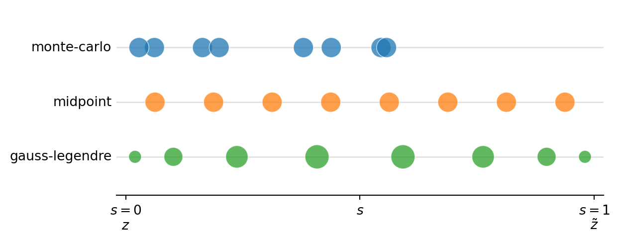
Midpoint cuts \([0,1]\) into \(N\) equal cells and evaluates at each centre, every node counting \(1/N\) — the even row of equal discs. Inside a cell the integrand’s slope tips the estimate one way to the left of the centre and the other way to the right, so the first-order error cancels and what survives is second order: the error scales as \(N^{-2}\). You can read this straight off the table below — every doubling of \(N\) divides the error by 4.
Gauss-legendre fixes neither. With \(2N\) free parameters — nodes and weights — the rule can be made exact for every polynomial of degree \(\le 2N-1\). That is why its discs are unequal and drift toward the endpoints: it is not sampling the segment, it is solving for the cheapest way to integrate a polynomial. When \(D\) is smooth, \(J_D\) along the segment is well approximated by one, and the error falls geometrically in \(N\) rather than polynomially — the cliff in the next figure. The optimal nodes are roots of Legendre polynomials on \([-1,1]\), hence the rescaling.
Monte-carlo throws the nodes down at random with equal weights, and the top row shows the price. All eight nodes fall below \(s \approx 0.56\); two of them sit \(0.012\) apart, very nearly the same Jacobian computed twice; and everything beyond — some \(44\%\) of the segment, the stretch nearest \(\tilde z\) — is never looked at. Nothing is wrong with the sampler, that is simply what eight uniform draws look like. The central limit theorem gives an error of \(\sigma/\sqrt N\) — a rate that does not depend on the dimension of the integral. That dimension-independence is what makes monte-carlo indispensable for high-dimensional expectations, and exactly what makes it pointless here: our integral is over a single scalar, so we pay the slow rate for a robustness we have no use for.
One caveat on gauss-legendre: its speed is borrowed from smoothness. Swap the tanh for a ReLU and \(J_D\) becomes piecewise constant with jumps along the segment — no polynomial fits it well, the geometric rate collapses, and the \(C^1\) assumption we opened with is gone anyway.
We compare the estimate \(\bar A \, \delta z\) against the true difference \(D(z + \delta z) - D(z)\), averaged over 10 random pairs, as a function of the number of Jacobian evaluations.
def mean_rel_error(rule, N, pairs):
    errs = []
    for z, dz in pairs:
        s, w = rule(N)
        true = D(z + dz) - D(z)
        errs.append((estimate_difference(z, dz, s, w) - true).norm() / true.norm())
    return torch.stack(errs).mean().item()


pairs = [(torch.randn(n), torch.randn(n)) for _ in range(10)]
rules = [("monte-carlo", nodes_monte_carlo),
         ("midpoint", nodes_midpoint),
         ("gauss-legendre", nodes_gauss_legendre)]
Ns = [1, 2, 4, 8, 16, 32, 64, 128, 256]

curves = {name: [mean_rel_error(rule, N, pairs) for N in Ns]
          for name, rule in rules}

print(f"{'N':>5} " + " ".join(f"{r:>15}" for r, _ in rules))
for i, N in enumerate(Ns):
    print(f"{N:>5} " + " ".join(f"{curves[r][i]:15.2e}" for r, _ in rules))
N monte-carlo midpoint gauss-legendre
1 4.80e-01 1.17e-01 1.17e-01
2 3.20e-01 2.30e-02 1.67e-02
4 2.62e-01 4.75e-03 4.63e-04
8 1.49e-01 1.16e-03 2.32e-06
16 9.06e-02 2.90e-04 3.06e-11
32 1.03e-01 7.23e-05 1.02e-15
64 3.08e-02 1.81e-05 9.67e-16
128 2.15e-02 4.52e-06 1.32e-15
256 3.21e-02 1.13e-06 1.67e-15fig, ax = plt.subplots(figsize=(7, 4.5))
for rule_name, _ in rules:
ax.loglog(Ns, np.clip(curves[rule_name], 1e-17, None), marker="o", label=rule_name)
ax.loglog(Ns, 0.3 / np.sqrt(Ns), "k--", lw=1, label=r"$1/\sqrt{N}$")
ax.set_xlabel("Jacobian evaluations $N$")
ax.set_ylabel("mean relative error")
ax.grid(alpha=.3)
ax.legend()
plt.tight_layout()
plt.show()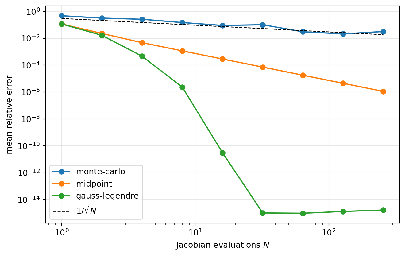
The identity is confirmed: gauss-legendre drives the error to machine precision (~\(10^{-15}\)) with about 32 Jacobian evaluations, and is already at \(10^{-11}\) with 16. The net is smooth, so the quadrature converges spectrally.
Monte-carlo is the loser, and by a wide margin. It sits on the \(1/\sqrt N\) line: 256 evaluations to still be around 3%, where midpoint is already near \(10^{-6}\) and gauss-legendre is at machine precision. It is also visibly noisy — the error is not even monotone in \(N\). For a one-dimensional integral, sampling is the wrong instinct; keep it only if you need the unbiasedness.
This is what \(\bar A\) buys over the tangent \(J_D(z)\). We fix a direction and grow \(\|\delta z\|\):
z = torch.randn(n)
direction = torch.randn(n)
direction /= direction.norm()
s, w = nodes_gauss_legendre(64)

print(f"{'||dz||':>8} {'path integral':>16} {'tangent J(z) dz':>18}")
for scale in [0.01, 0.1, 0.5, 1.0, 2.0, 4.0]:
    dz = scale * direction
    true = D(z + dz) - D(z)
    e_path = (estimate_difference(z, dz, s, w) - true).norm() / true.norm()
    e_tan = (jacrev(D)(z) @ dz - true).norm() / true.norm()
    print(f"{scale:8.2f} {e_path:16.1e} {e_tan:18.1e}")
||dz|| path integral tangent J(z) dz
0.01 1.8e-13 3.8e-03
0.10 2.2e-14 3.9e-02
0.50 3.1e-15 1.9e-01
1.00 2.2e-15 3.1e-01
2.00 1.1e-15 7.3e-01
4.00 9.7e-16 1.0e+00The tangent linearisation degrades exactly as expected, its error growing with the step size until it is meaningless. The path integral stays at machine precision no matter how far apart the two points are — which is the entire content of the trick.